Regression Modeling with Azure Machine Learning Studio
Sep 8, 2020 • 10 Minute Read
Introduction
Regression modeling is one of the most widely used machine learning algorithms. It is used in predictive modeling when the target variable is continuous. In this guide, you will learn how to perform regression modeling with Azure Machine Learning Studio.
Data
In this guide, you will work with US economic time series data available from https://research.stlouisfed.org/fred2. The data contains 574 rows and five variables, as described below:
-
psavert Personal savings rate.
-
pce Personal consumption expenditures, in billions of dollars.
-
uempmed Median duration of unemployment, in weeks.
-
pop Total population, in thousands.
-
unemploy Number of unemployed in thousands. This is the dependent variable.
Start by loading the data.
Loading Data
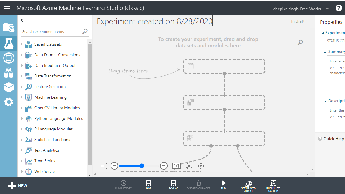
Once you have logged into your Azure Machine Learning Studio account, click on the EXPERIMENTS option, listed on the left sidebar, followed by the NEW button. Next, click on the blank experiment and the following screen will be displayed.
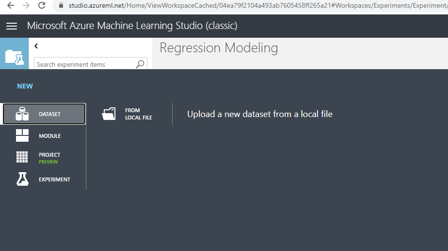
Give the name "Regression Modeling" to the workspace. Next you will load the data into the workspace. Click NEW, and select the DATASET option shown below.
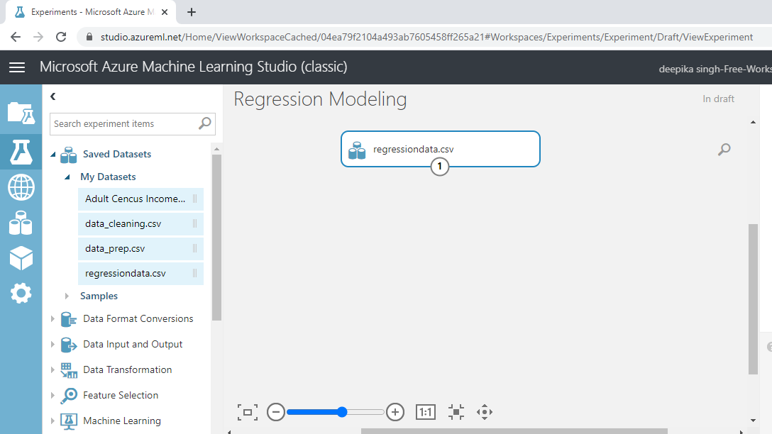
The selection above will open a window that can be used to upload the dataset from the local system. Upload the data named regressiondata.csv. Once the file is loaded, you can see it in the Saved Datasets option. The next step is to drag it from the Saved Datasets list into the workspace.
Exploring the Data
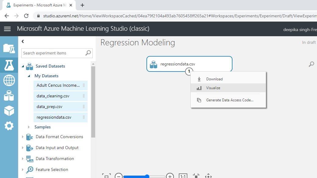
Exploring the data is important because it helps you understand the data and prepare it for further analysis. To explore the data, right-click and select the Visualize option.
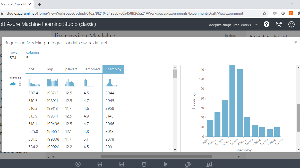
Select the different variables to examine the basic statistics. For example, the image below displays the details for the target variable unemploy.
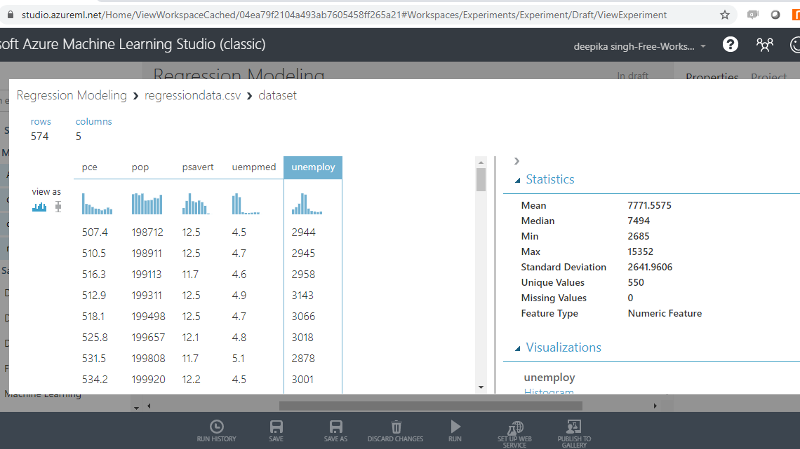
The Statistics section on the right-hand side displays summary statistic values for the variable. If you scroll down the workspace, you can see the histogram. The summary statistic and the histogram enables you understand the distribution of the variable.
Create, Train, and Test Datasets
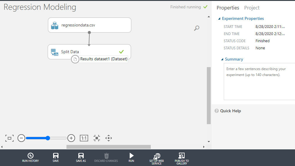
It is important to validate the performance of the machine learning model being built. To do that, one of the approaches is to divide the data into training and test data. This is done with the Split Data module. Search and drag the module into the workspace.
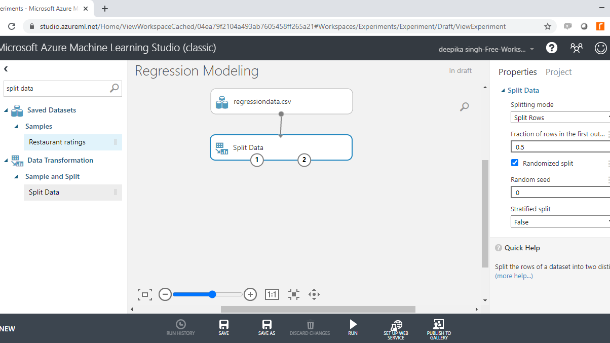
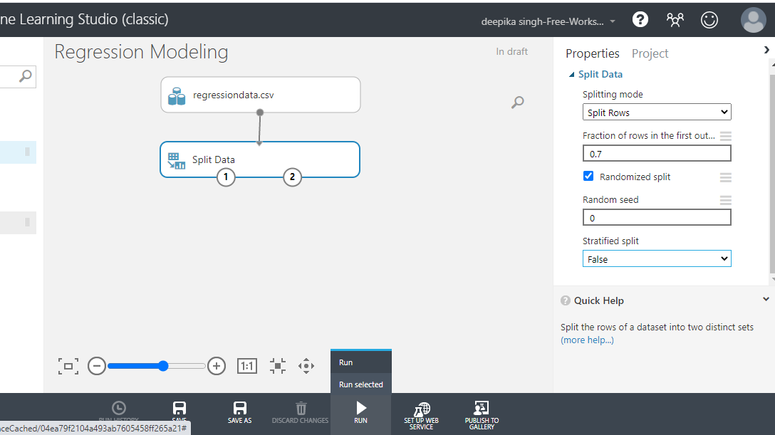
In the Split Data options displayed in the right-hand side of the workspace, change the value under the tab Fraction of rows in the first to 0.7. This means you are keeping 70% of the data in the training set, while the remaining 30% will remain in the test set. Next, click on the Run tab and select Run selected.
Once the module run is completed, you can locate the training date on the left output port as Results dataset1.
Right click and select the Visualize option.
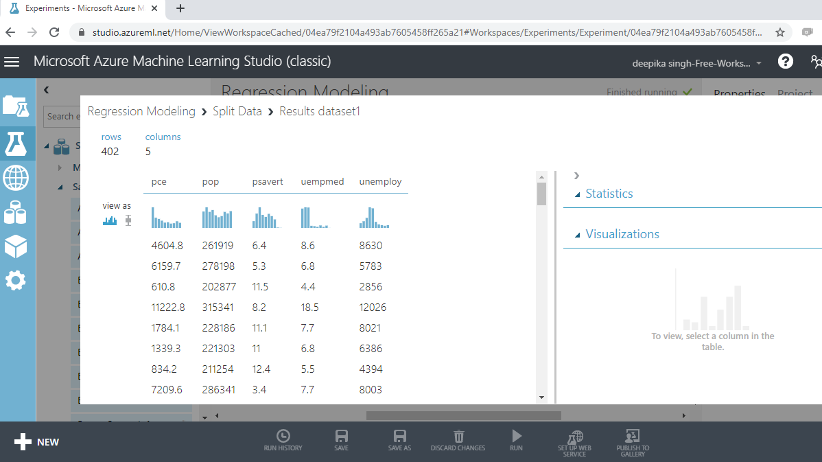
The output above shows that there are 402 rows and five columns in the training dataset, which represent 70% of the data.
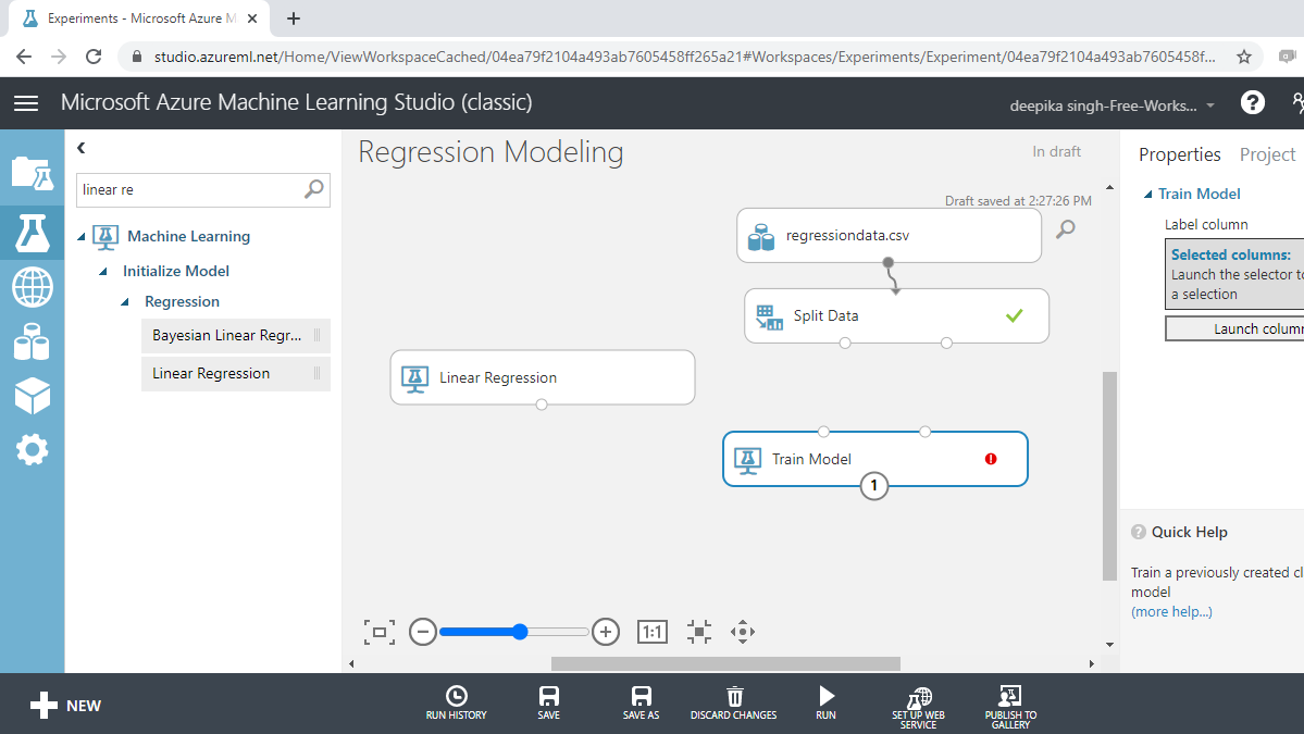
Train the Model
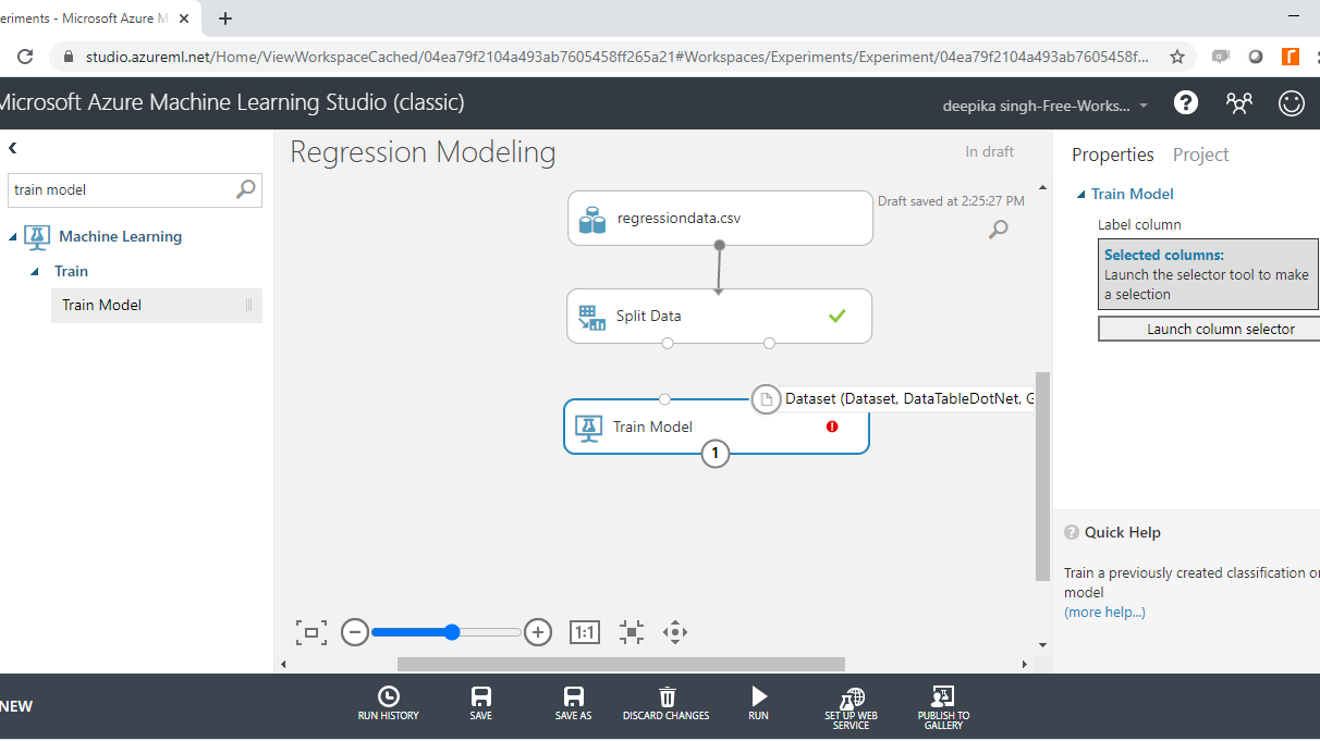
Drag the Train Model module into the workspace as shown below. The module has two input ports. The first port is for Untrained model that will connect with the algorithm module.
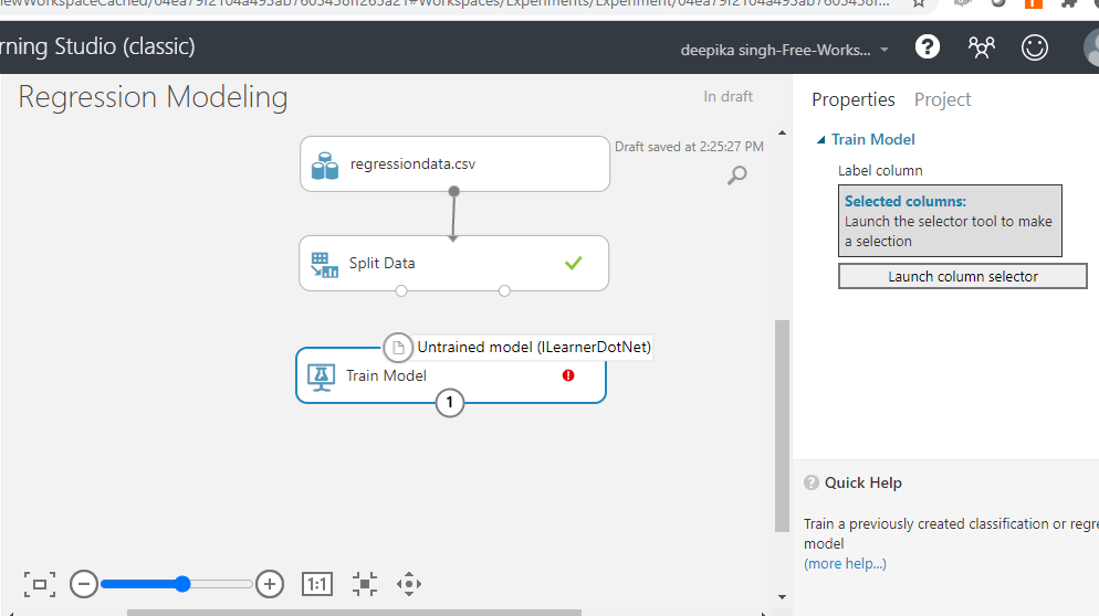
The second port is the Dataset port.
The next step is to add the machine learning module into the workspace. Since the target variable is continuous, you will build a regression model. There are many regression algorithms available in Azure Machine Learning Studio. You will select and drag the Linear Regression module into the workspace.
Linear Regression
Multiple linear regression is a supervised machine learning algorithm, which assumes that the independent variables have a linear relationship with the dependent variable. Also, the input variables are assumed to have a Gaussian distribution, which is required for a random variable to have normal distribution. Another assumption is that the predictors are not highly correlated with each other (a problem called multi-collinearity).
The next step is to set up the workspace for training the model as shown below.
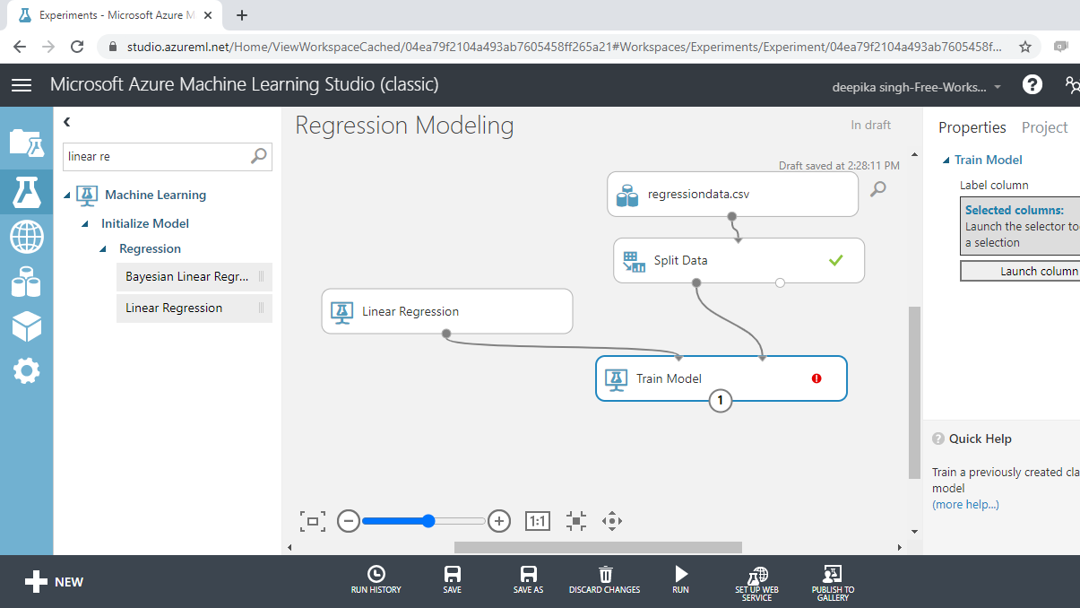
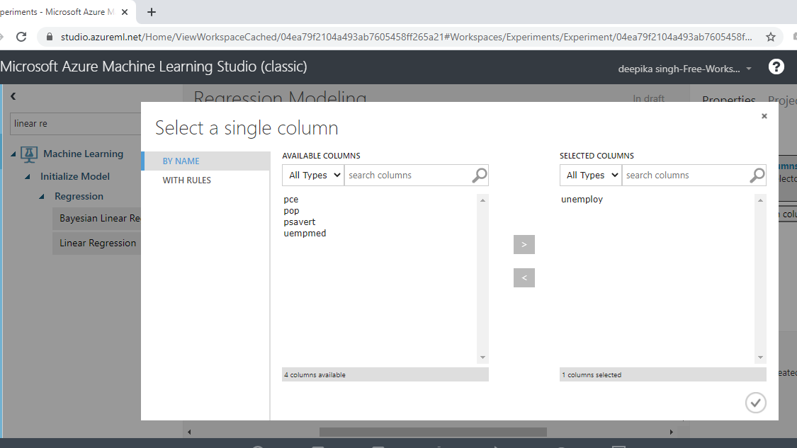
In the output above, you can see that there is a red circle inside the Train Model module which indicates that the setup is not complete. This is because the target variable is not yet specified. To do this, click on Launch column selector, and place the target variable unemploy into the selected columns box, as shown below.
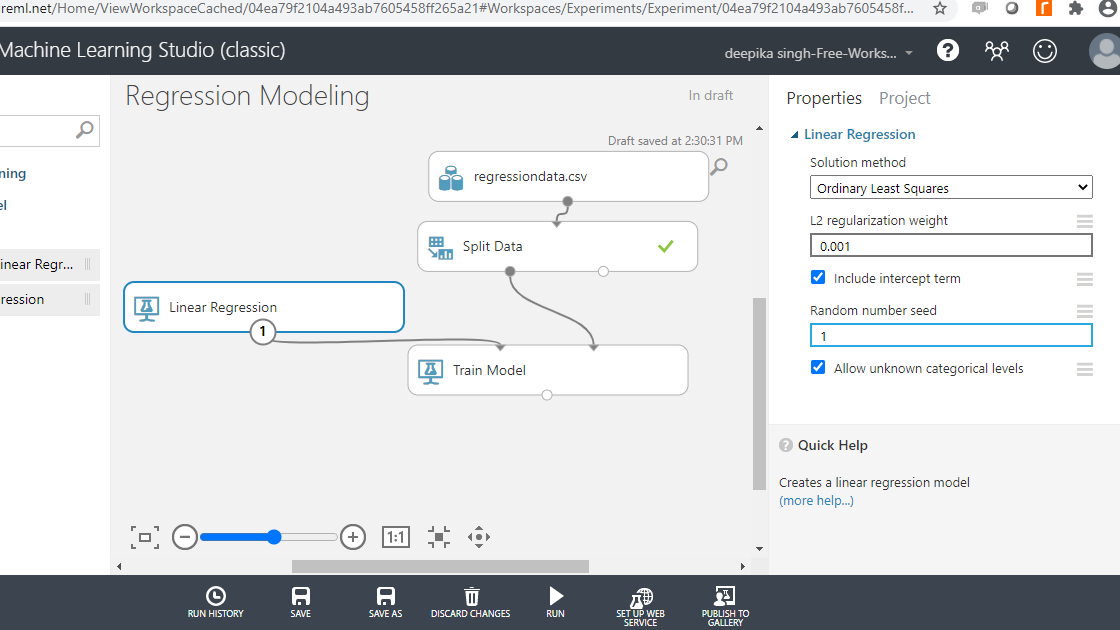
Parameter Specification
The next step is to specify the parameters of the algorithm. This step is required for the model to understand how it is supposed to train the algorithm. To start, click on the Linear Regression module and fill in the details of your choice under the Properties pane.
Choose the Ordinary Least Squares option under the Solution method pane. The ordinary least squares method is one of the most commonly used techniques in linear regression, and it works by minimizing the sum of squares of residuals (actual value - predicted value). The second input is for L2 regularization weight. This is used to prevent model overfitting, and a non-zero value is preferred.
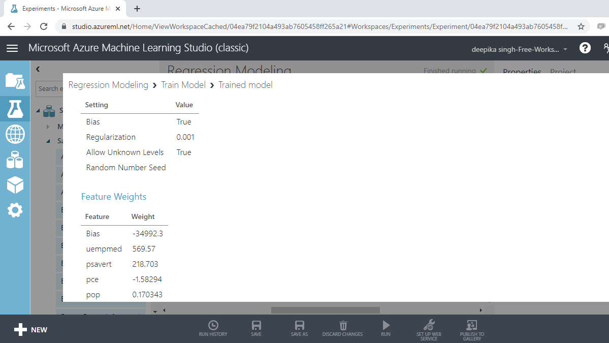
The next step is to click on the RUN tab to run the experiment, followed by visualizing the trained model.
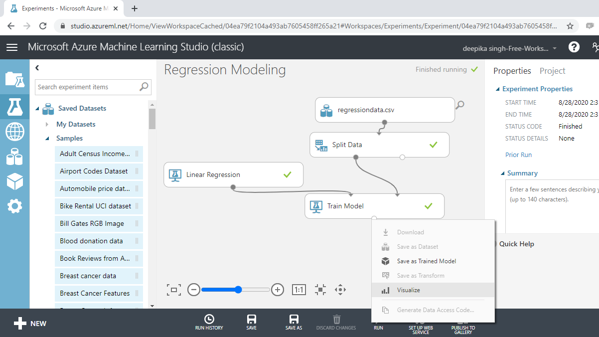
Completing the above step will produce the following output which shows the model details and the feature weights.
Score Test Data
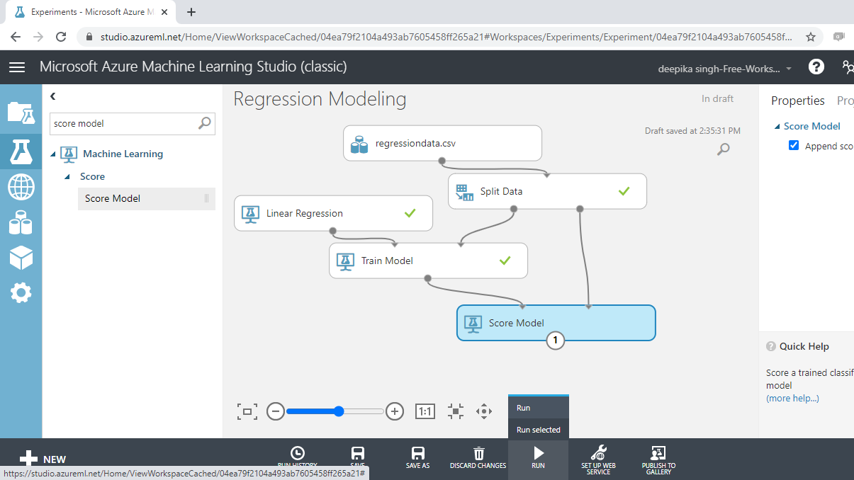
The model has been built and the next step is to score the test data. This step is the pre-requisite for model evaluation. To do this, perform the following steps.
-
Drag the Score Model module into the workspace.
-
Connect the output port of the Train Model with the left input port of the Score Model module.
-
Connect the right output port of the Split Data module to the right input port of the Score Model module. Note that this connects the test data in the Split Data module with the scoring function.
Click on RUN and select Run selected. Your workspace will look as below.
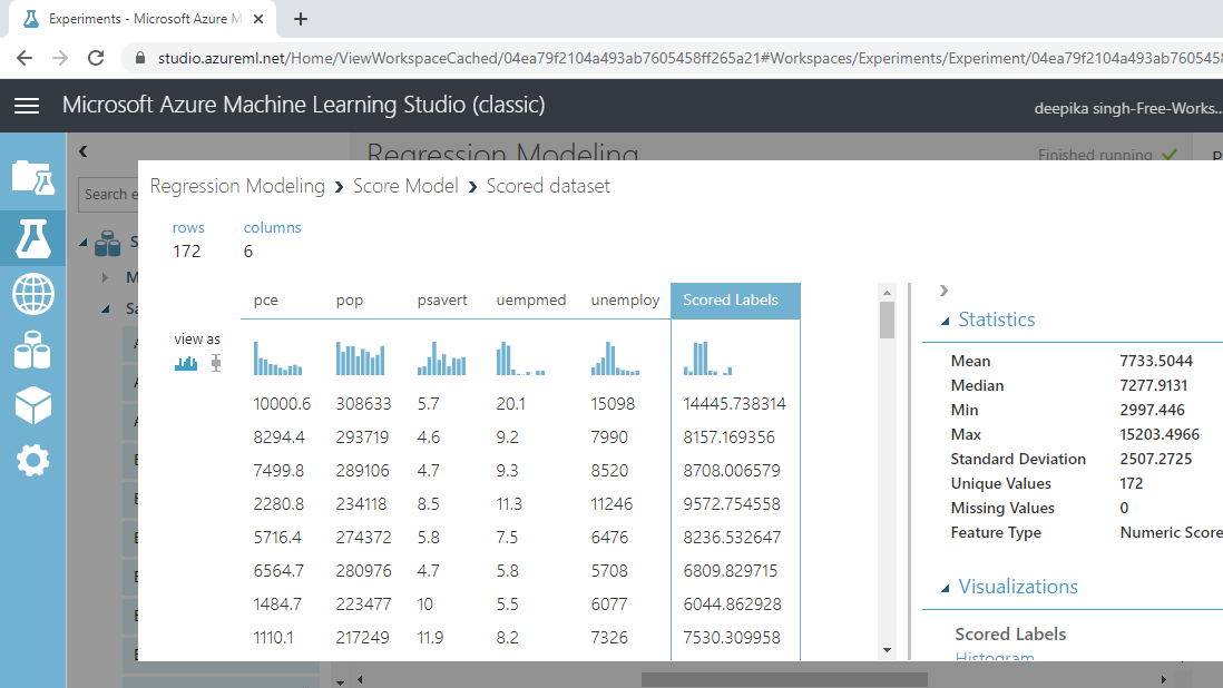
To look at the scored results, click on the Visualize option.
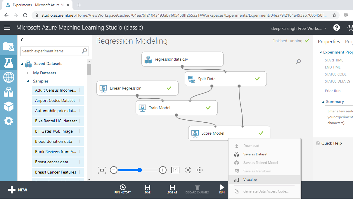
The new variable, Scored Labels, displays the predictions on the test data. This is shown below.
Evaluate the Model
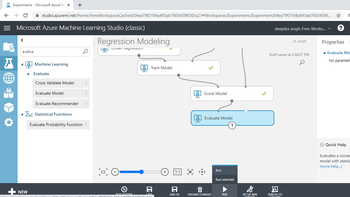
You have built the predictive model and generated predictions on the test data. The next step is to evaluate the performance of your predictive model. Drag the Evaluate Model module into the workspace and connect it with the Score Model module. Next, click on the Run tab and select Run selected. This is shown below.
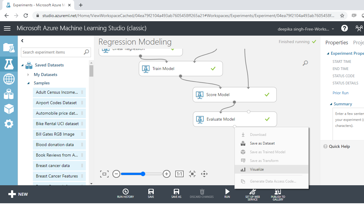
Next, right click on the output port of the Evaluate Model module and click on the Visualize option.
The result window will open, and you can look at the evaluation metrics for regression model.
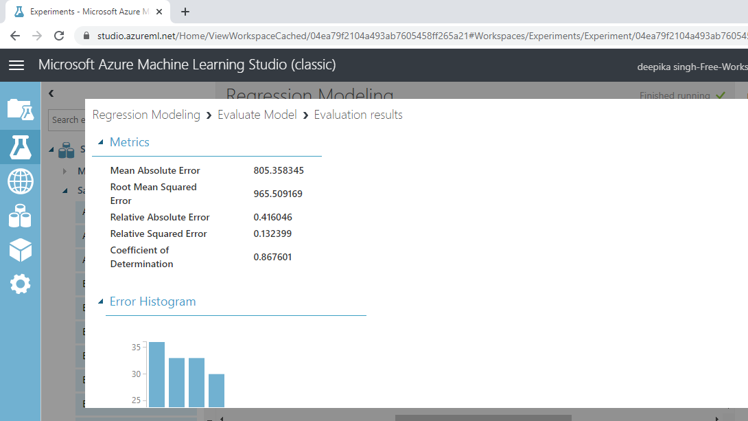
The output above shows that the coefficient of determination, or the R-squared value, is 87%, which is good model performance.
Conclusion
In this guide, you learned how to perform regression modeling in Azure Machine Learning Studio. You learned how to load the data set from your computer system into the ML Studio, and then build, score, and evaluate a regression model.
To learn more about data science and machine learning using Azure Machine Learning Studio, please refer to the following guides: