Build Your First Image Classification Experiment

Jun 17, 2020 • 13 Minute Read

Introduction

Working knowledge of neural networks, TensorFlow and image classification are essential tools in the arsenal of any data scientist, even for those whose area of application is outside of computer vision. Indeed, the technology of Convolutional Neural Networks (CNNs) has found applications in areas ranging from speech recognition to malware detection and even to understanding climate. This guide will help you onboard onto using these tools at lightning speed by guiding you through a fun starter project of classifying cats and dogs, and then point the way to subsequent steps to becoming an expert on image classification.

Code for this guide is available on Github.

Accessing the Dataset

If you haven’t registered yet to Kaggle, head on over to Kaggle and create an account. Open the settings to your account and click Create New API Token:

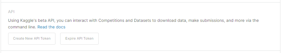
This will download a Kaggle API json file, which you’ll want to place at ~/.kaggle/kaggle.json (or, for a typical Windows setup, at C:\Users\<Windows-username>\.kaggle\kaggle.json).

The Kaggle API is a convenient way to access datasets. For more information on Kaggle’s API, see Kaggle API Github page.

If your environment lacks the Kaggle pip library, install it by running:

      pip install kaggle

Now, you can use the Kaggle APIs. In your environment, run:

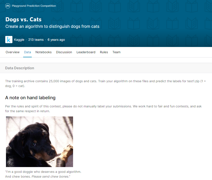
      kaggle competitions download -c dogs-vs-cats

This will download the “Dogs vs. Cats” dataset.

Next, you will unzip the dataset and, for clarity, remove unneeded data.

      !unzip train.zip
!mv train data
!rm test1.zip sampleSubmission.csv train.zip
    

You now have a dataset consisting of cat and dog images.

Exploring the Data

Next, you’ll perform some data exploration. Set a variable pointing to the dataset’s location.

      DATASET_LOCATION = "data"

Collect the labels and filenames of the dataset.

      import os

filenames = os.listdir(DATASET_LOCATION)
classes = []
for filename in filenames:
    image_class = filename.split(".")[0]
    if image_class == "dog":
        classes.append(1)
    else:
        classes.append(0)
    

Read the dataset into a pandas dataframe for convenient access.

      import pandas as pd

df = pd.DataFrame({"filename": filenames, "category": classes})
df["category"] = df["category"].replace({0: "cat", 1: "dog"})
    

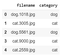
You can see you now have labels for the files:

      df.head()

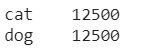
In addition, you can see that the dataset is balanced, and consists of 12,500 images of cats and dogs, each:

      df.category.value_counts()

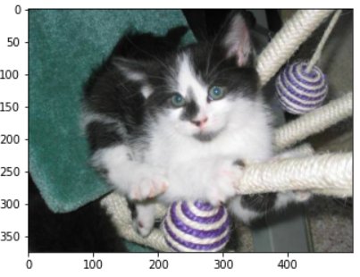
The following code block will display a random image:

      import random
from keras.preprocessing.image import load_img
import matplotlib.pyplot as plt

sample1 = random.choice(filenames)
image1 = load_img(DATASET_LOCATION + "/" + sample1)
plt.imshow(image1)
    

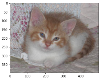
Here is code to preview another datapoint:

      sample2 = random.choice(filenames)
image2 = load_img(DATASET_LOCATION + "/" + sample2)
plt.imshow(image2)
    

The sizes of the images are not uniform:

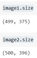
This is important because for a standard neural network classifier, the sizes of the inputs must be identical. Fortunately, this is not a problem, as you will rescale all images to the same size. Specify the desired size:

      IMAGE_WIDTH = 64
IMAGE_HEIGHT = 64
IMAGE_SIZE = (IMAGE_WIDTH, IMAGE_HEIGHT)
INPUT_SHAPE = (IMAGE_WIDTH, IMAGE_HEIGHT, 1)
    

You now have a good sense of what the dataset consists of.

Instantiating a Convolutional Neural Network (CNN) Classifier

Next, you will specify the architecture of a neural network that you will use to classify the images. The architecture you will use is a simple, standard CNN meant to serve as a starting point. The library that implements the CNN is called Keras, and is a high-level API that can use lower-level neural network libraries, such as TensorFlow, under the hood.

      import keras
from keras.models import Sequential
from keras.layers import Dense, Dropout, Flatten
from keras.layers import Conv2D, MaxPooling2D

model = Sequential()
model.add(Conv2D(32, kernel_size=(3, 3), activation="relu", input_shape=INPUT_SHAPE))
model.add(Conv2D(64, (3, 3), activation="relu"))
model.add(MaxPooling2D(pool_size=(2, 2)))
model.add(Dropout(0.25))
model.add(Flatten())
model.add(Dense(128, activation="relu"))
model.add(Dropout(0.5))
model.add(Dense(2, activation="softmax"))

model.compile(
    loss=keras.losses.categorical_crossentropy,
    optimizer=keras.optimizers.Adadelta(),
    metrics=["accuracy"],
)
    

The model consists of convolutional layers, max pooling layers, dense layers and dropout layers. It utilizes categorical cross-entropy as a loss function, and Adadelta as its optimizer.

Preprocessing the Dataset

To train the model on the data, and to be able to assess its performance as it trains, split the dataset into a training and testing set:

      from sklearn.model_selection import train_test_split

train_df, test_df = train_test_split(df, test_size=0.20, random_state=42)

Keras also has very convenient methods to perform data augmentation and reading images from directories. Data augmentation is a procedure in which existing data is used to generate new data. For example, you can take an existing image and flip it to create another data point. That is what an ImageDataGenerator allows you to do.

      from keras.preprocessing.image import ImageDataGenerator

train_datagen = ImageDataGenerator(
    rotation_range=15,
    rescale=1.0 / 255,
    shear_range=0.1,
    zoom_range=0.2,
    horizontal_flip=True,
    width_shift_range=0.1,
    height_shift_range=0.1,
)
    

The flow_from_dataframe method efficiently reads and preprocesses files of a directory.

      BATCH_SIZE = 16
train_generator = train_datagen.flow_from_dataframe(
    train_df,
    DATASET_LOCATION,
    x_col="filename",
    y_col="category",
    target_size=IMAGE_SIZE,
    class_mode="categorical",
    batch_size=BATCH_SIZE,
    color_mode="grayscale",
)
    

Create a similar generator for the test images

For illustrative purposes, create a generator for a single image and display the corresponding augmented data.

      example_df = train_df.sample(n=1)
example_generator = train_datagen.flow_from_dataframe(
    example_df,
    DATASET_LOCATION,
    x_col="filename",
    y_col="category",
    target_size=IMAGE_SIZE,
    class_mode="categorical",
    color_mode="grayscale",
)
    

Plot the augmented data.

      plt.figure(figsize=(12, 12))
for i in range(0, 15):
    plt.subplot(5, 3, i + 1)
    for X_batch, Y_batch in example_generator:
        image = X_batch[0]
        image = image.reshape(IMAGE_SIZE)
        plt.imshow(image)
        break
plt.tight_layout()
plt.show()
    

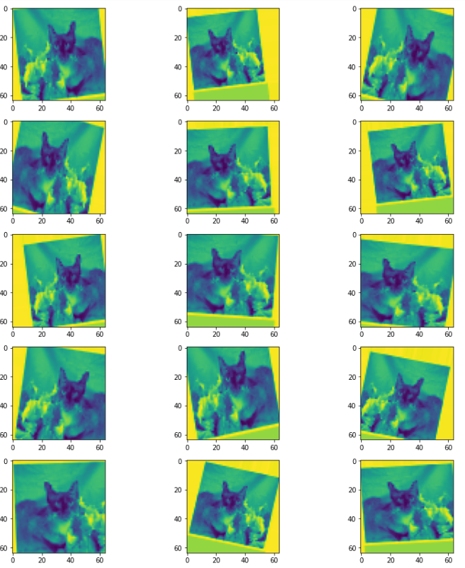
Note that throughout, you have greyscaled the data. The purpose of this is to reduce the size of the data, and therefore the corresponding computational burden. You have now setup the data preprocessing part of your training pipeline.

Training the CNN Using a GPU

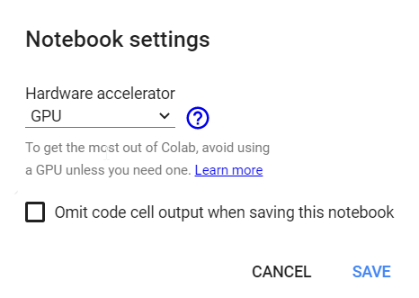
If you have access to a GPU, this is the time to enable it. A GPU accelerates most Deep Learning computations (i.e., computations for neural networks with many layers). If you are using a Google Colab notebook, click on Runtime and then on Change runtime type. Under Hardware accelerator, select GPU and then SAVE.

You now are running your notebook with a GPU enabled. Go ahead and train your model .

      EPOCHS = 10
history = model.fit_generator(
    train_generator,
    epochs=EPOCHS,
    validation_data=test_generator,
    validation_steps=test_df.shape[0] // BATCH_SIZE,
    steps_per_epoch=train_df.shape[0] // BATCH_SIZE,
)
    

This might take a bit of time, but with the simplifications you have made, such as small greyscale images, it shouldn’t be much longer than 10 minutes. Once finished, you should see something like this:

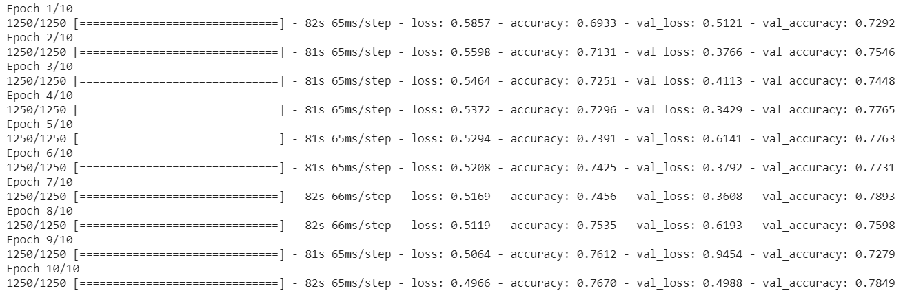
Looking at val_accuracy, you can see that the classifier attains about 78% accuracy on the testing set, which is a good starting point for further improvements. Looking at the accuracy, which is the training accuracy, you can see that it stays close to the val_accuracy. The implication is that your network is not overfitting, meaning that it is not inferring rules that aren't true. You will see suggestions for improvement in a later section.

It’s nice to see the classifier in action. Take some six samples to observe:

      NUM_SAMPLES = 6
sample_test_df = test_df.head(NUM_SAMPLES).reset_index(drop=True)
sample_test_datagen = ImageDataGenerator(rescale=1.0 / 255)
sample_test_generator = sample_test_datagen.flow_from_dataframe(
    sample_test_df,
    DATASET_LOCATION,
    x_col="filename",
    y_col="category",
    target_size=IMAGE_SIZE,
    class_mode="categorical",
    batch_size=BATCH_SIZE,
    color_mode="grayscale",
)
    

Predict on these samples:

      predict = model.predict_generator(sample_test_generator)
import numpy as np

predictions = np.argmax(predict, axis=-1)
    

And display the results:

      plt.figure(figsize=(12, 24))
for index, row in sample_test_df.iterrows():
    filename = row["filename"]
    prediction = predictions[index]
    img = load_img(DATASET_LOCATION + "/" + filename)
    plt.subplot(6, 3, index + 1)
    plt.imshow(img)
    plt.xlabel(prediction)
plt.tight_layout()
plt.show()
    

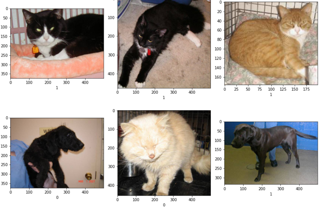
As you can see, the classifier performs with some mistakes. But that's okay for a first prototype.

Conclusion

You have accomplished much in this guide, taking a set of images and constructing a classifier that can recognize these as images of cats or dogs. There is also a lot of exciting content to learn, from transfer learning to segmentation, in your path to expertise in image classification. Following the directions below, you will reach your destination in no time.

Improving Your Current Classifier

The following steps will yield improvements to your classifier on this problem:

Since the classifier is not overfitting it makes sense to experiment with training it for longer
Add additional layers to the network
Incorporate all three color channels of images
Perform additional data augmentation
Perform a hyperparameter search
Apply transfer learning (e.g., start with a pre-trained professionally-made model like VGG16 and use it on this problem). You can learn this technique in the course Building Image Classification Solutions Using Keras and Transfer Learning.

Additional Ways You Can Practice and Hone Your Skills of Image Classification

Working on different problems like these will allow you to expand the variety of problems you can solve:

Construct a classifier on a multi-class dataset
Perform object detection (finding an instance of some object within an image)
Apply segmentation. You can learn this technique in the course Implementing Image Recognition Systems with TensorFlow .

Happy learning!