Data Preprocessing with Azure ML Studio

Data preprocessing is an important data science activity for building robust and powerful machine learning models. It helps improve the data quality for modeling and results in better model performance. In this guide, you will learn how to treat outliers, create bins for numerical variables, and normalize data in Azure ML Studio.

In this guide, you will work with fictitious data of 600 observations and six variables, as described below.

1. Dependents - Number of dependents of the applicant.

2. Income - Annual Income of the applicant (in US dollars).

3. Loan_amount - Loan amount (in US dollars) for which the application was submitted.

4. Credit_score - Whether the applicant's credit score was good ("Satisfactory") or not ("Not_satisfactory").

5. Age - The applicant’s age in years.

6. approval_status - Whether the loan application was approved ("1") or not ("0"). This is the dependent variable.

Start by loading the data.

Once you have logged into your Azure Machine Learning Studio account, you will see the following window.

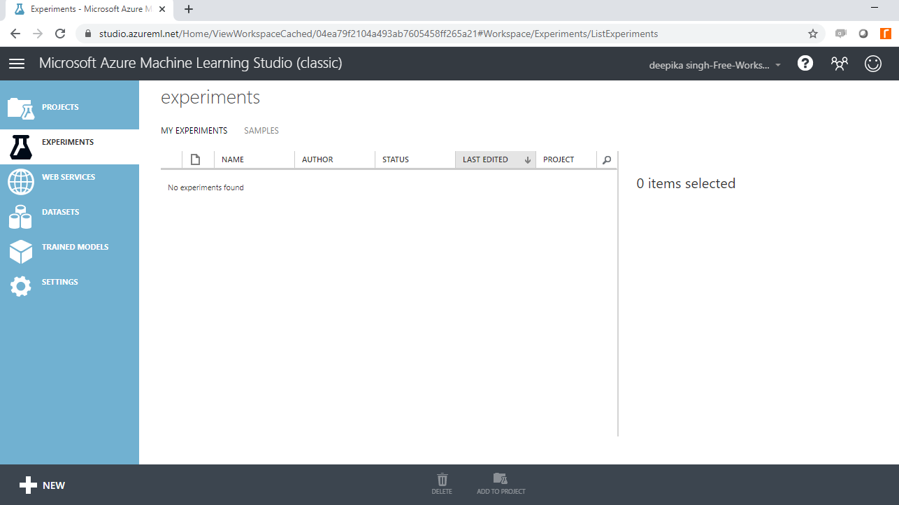
To start, click on the EXPERIMENTS option, listed on the left sidebar, followed by the NEW button. Next, click on the blank experiment, and the following screen will be displayed.

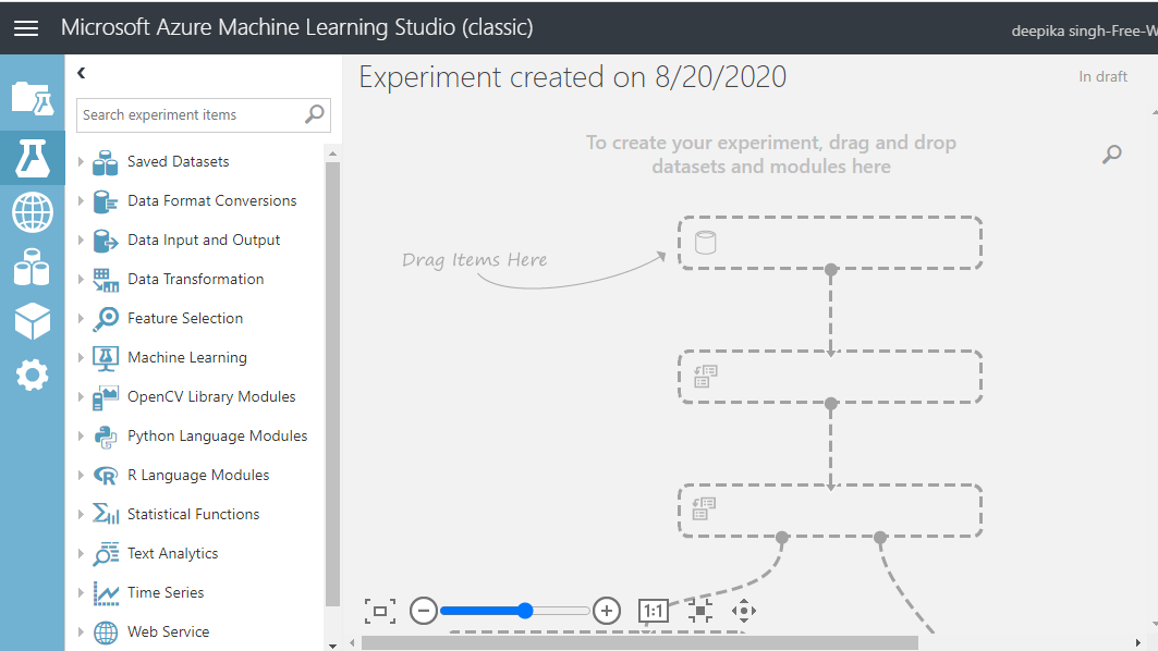
Give the name Experiment to the workspace. Next, load the data into the workspace. Click NEW, and select the DATASET option shown below.

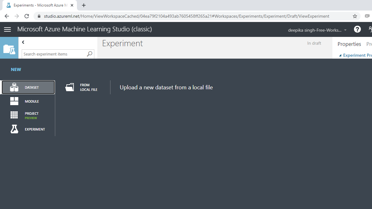
The selection above will open a window, shown below, which can be used to upload the dataset from the local system.

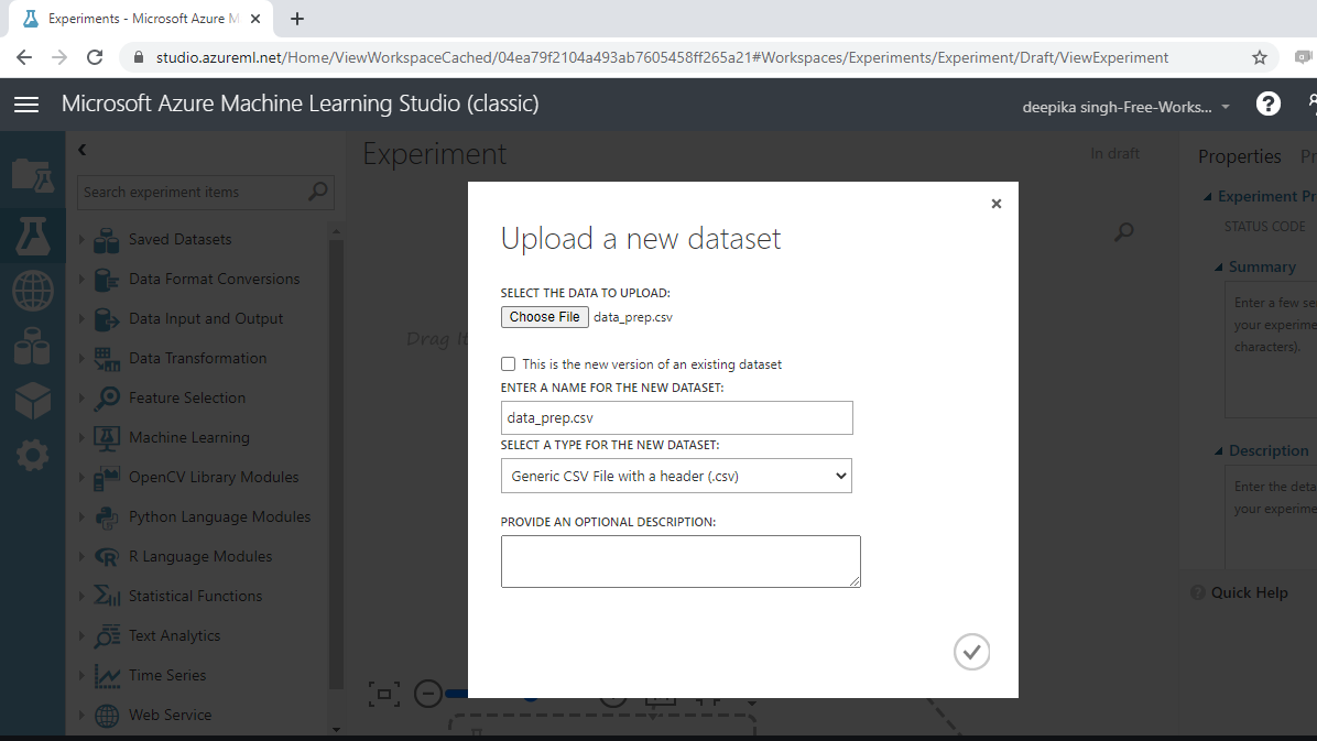
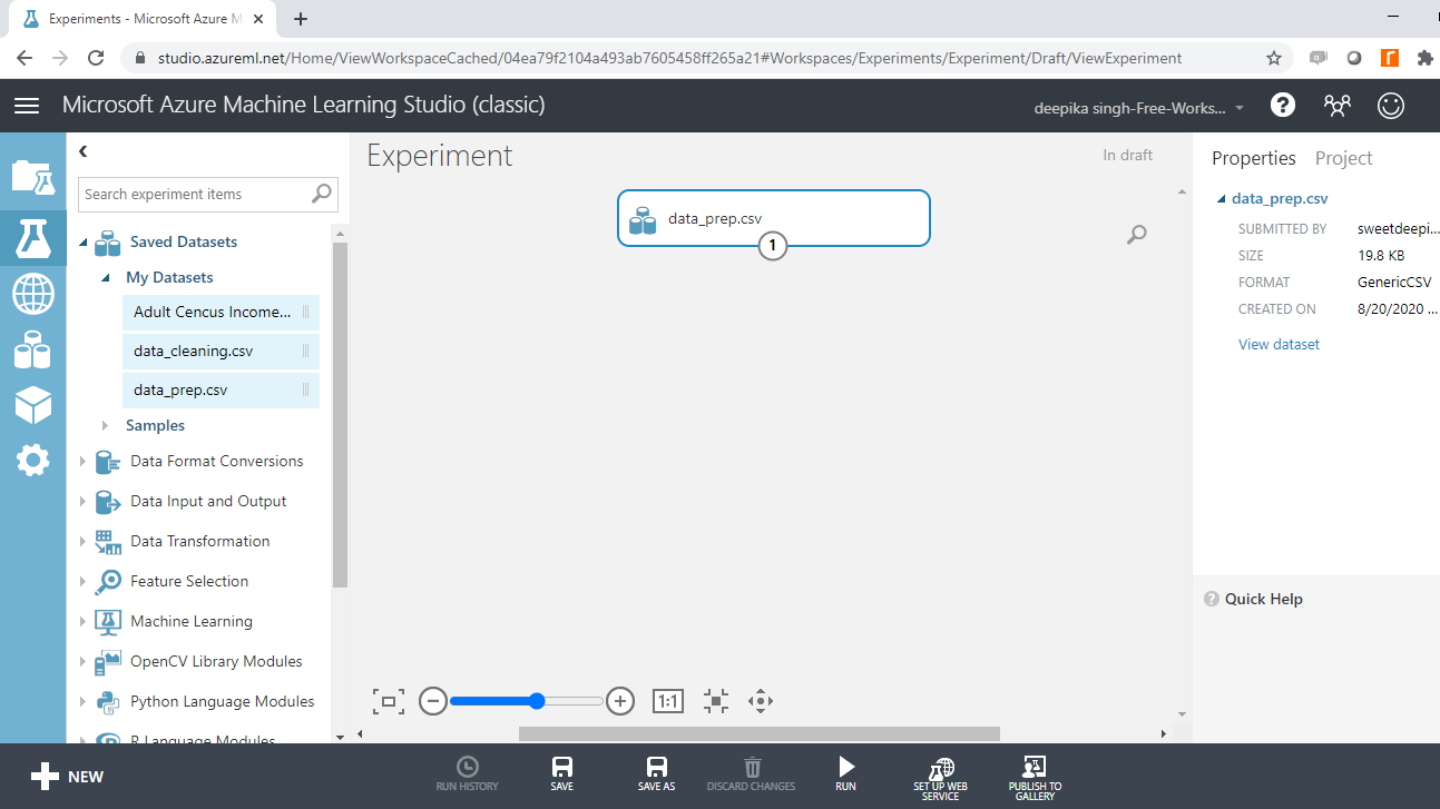
Once the data is loaded, you can see it in the Saved Datasets option. The file name is data_prep.csv. The next step is to drag it from the Saved Datasets list into the workspace.

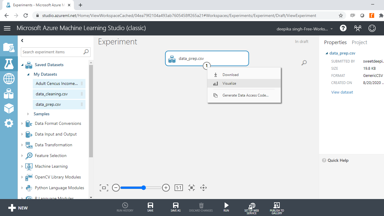
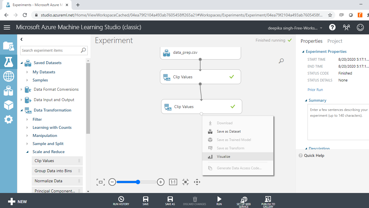
To explore the data, right-click and select the Visualize option as shown below.

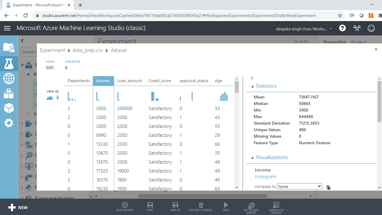
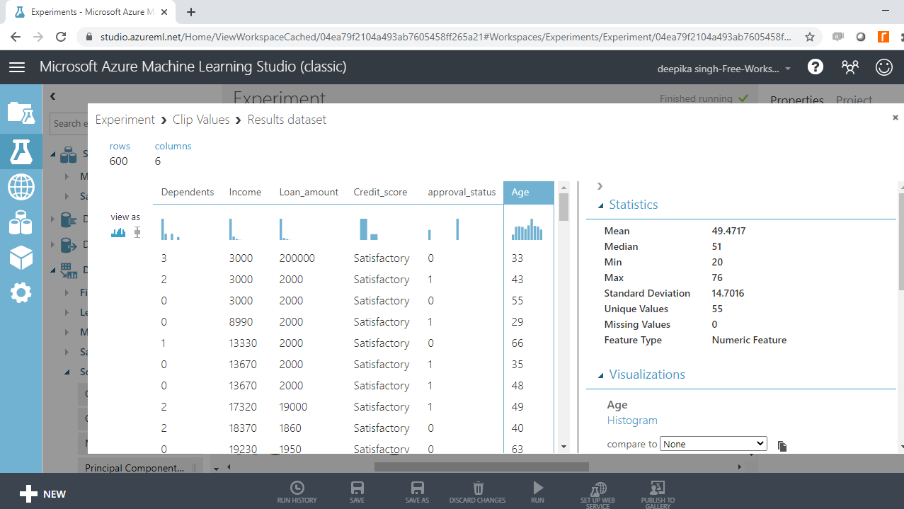
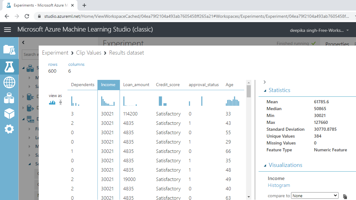
Select the different variables to examine the basic statistics. For example, the image below displays the details for the variable Age.

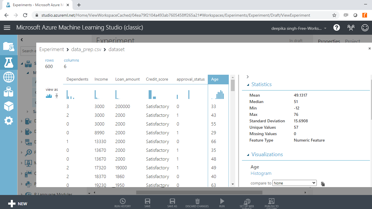
You will notice that the minimum value of age is -12, which indicates the presence of incorrect records in the data.

Next, look at the variables Loan_amount and Income.

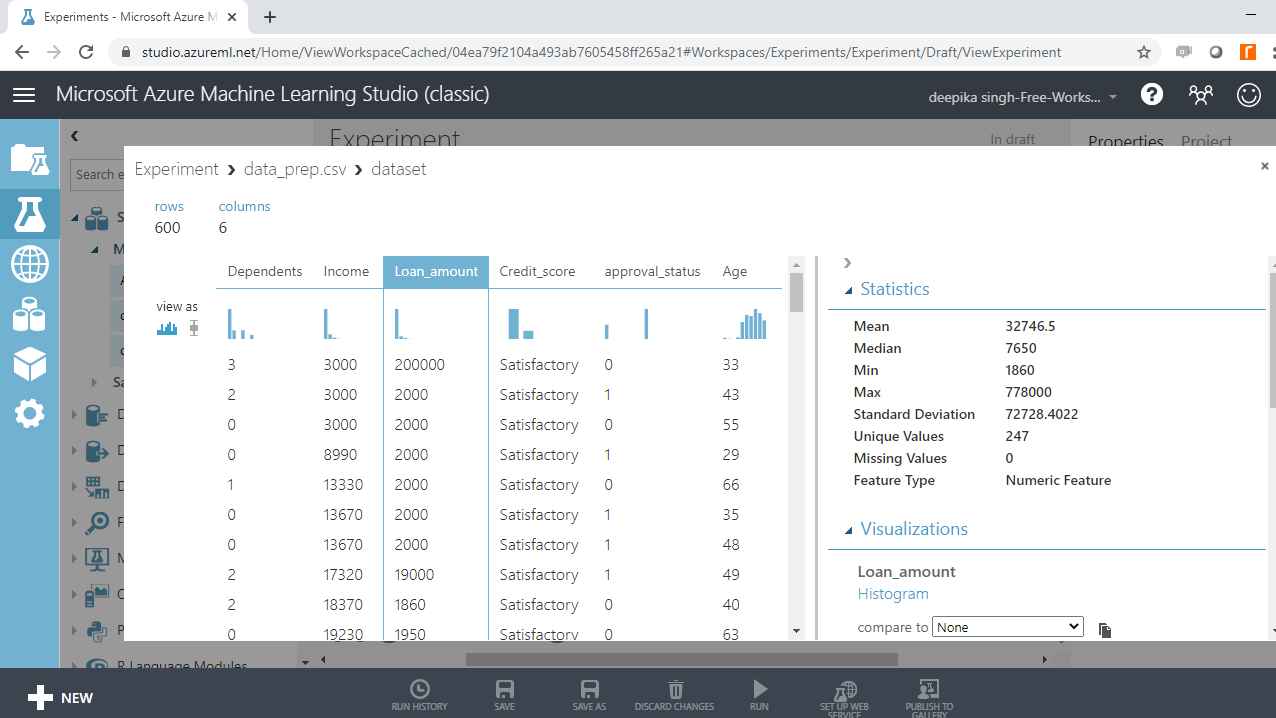
Both the outputs above show the presence of outliers in the variables. You will be dealing with these in subsequent sections.

You know from the above analysis that the variable Age has incorrect records. To treat this inconsistency, one method is to clip the values with the Clip Values module, which is used to identify and optionally replace data values that are above or below a specified threshold.

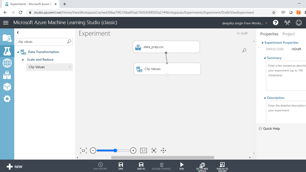
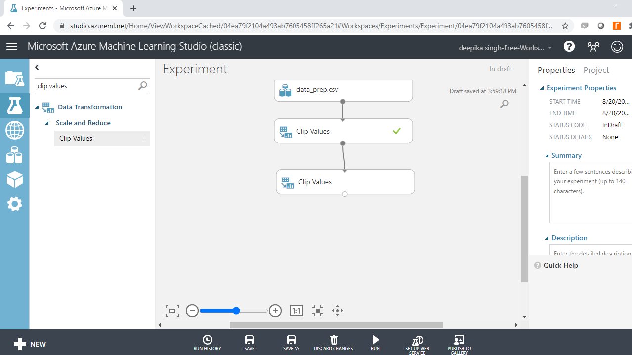
Start by entering clip values in the search bar to find the Clip Values module, and then drag it in the workspace as shown below.

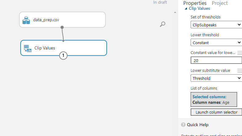
Next, click on Launch column selector to select the column that will be used to identify duplicates. This can be found in the Properties pane. Select the variable Age.

The next step is to set up the Clip Values module. The ClipSubpeaks option specifies the lower boundary. Values that are lower than the boundary value are replaced or removed. In this case, keep the lower value at 20. This means that the minimum value for age will be 20. Once the setup is done, click Run.

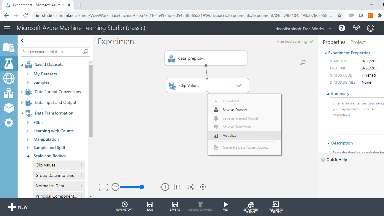
To check the results of the previous step, click Visualize.

Next, select the Age variable and you will see that the negative values have been replaced. The new subpeak value for age is twenty years.

One of the other obstacles in predictive modeling is the presence of outliers, which are extreme values that are different from the other data points. Outliers are often a problem because they mislead the training process and lead to inaccurate models. You can identify outliers visually through a histogram or numerically through the summary statistic value.

While exploring the data, you observed that the Income and Loan_amount variables had outliers. To start outlier treatment, drag the Clip Values module into the workspace as shown below.

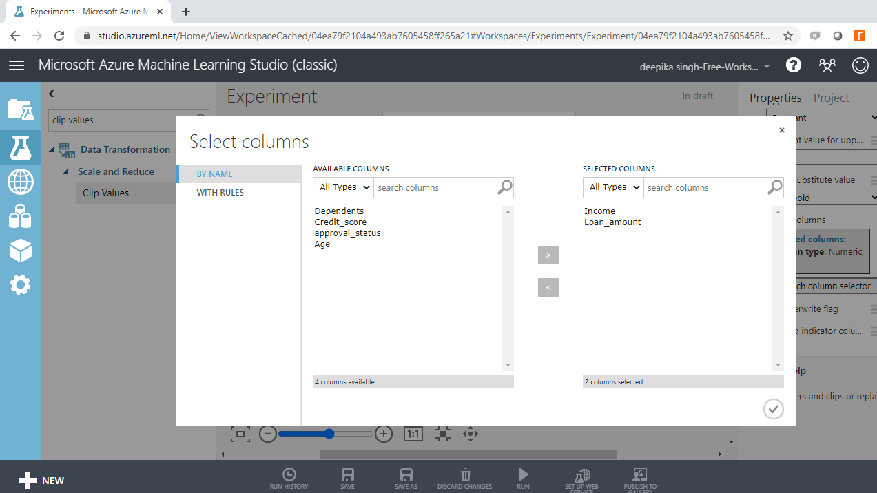
Click Launch column selector and select the two variables.

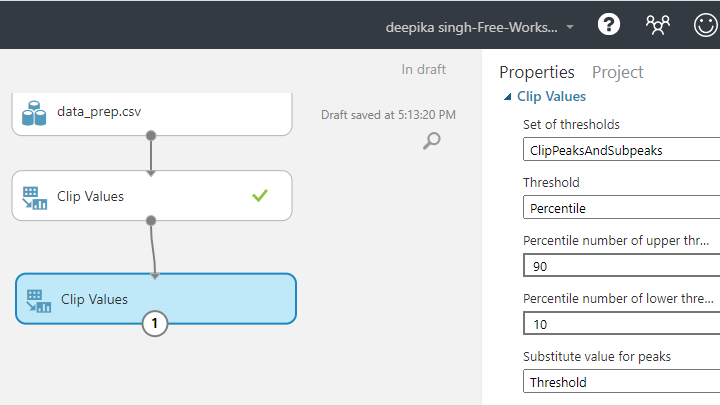
In the Properties pane, make the following arguments in the options.

1. For Set of thresholds, select the ClipPeaksAndSubpeaks option. This will specify both the upper and lower boundaries.

2. For Threshold, select the percentile option. This will specify the values to a percentile range.

3. Set Percentile value of lower threshold to 10 and Percentile value of upper threshold to 90. This will mean that values below and above these thresholds will be replaced by the tenth and ninetieth percentile values, respectively.

Once the setup is done, click on Run selected option shown below.

To check the results of the above transformation, right-click on the output port and select Visualize.

Click on the Income variable and check the result. The summary statistic values indicate that the mean and median values are now closer, and the standard deviation has come down from $71,213 to $30,771.

You have removed the outliers, but the numerical variables have different units, such as Age in years and Income in dollars. When the features use different scales, the features with larger scales can unduly influence the model. As a result, it is important to normalize the data. The goal of normalization is to change the values of numeric columns to use a common scale. Normalization is also required for some algorithms to model the data correctly.

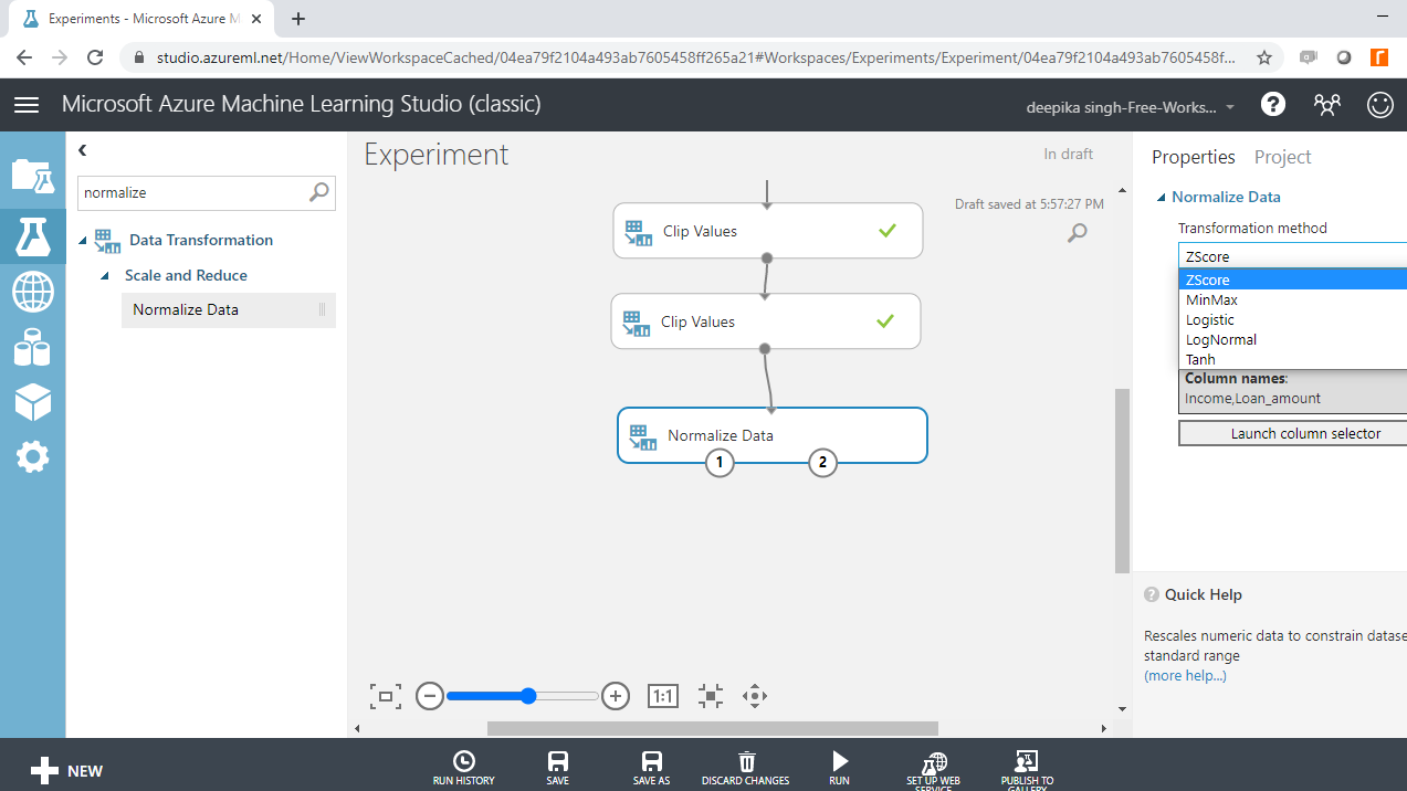
To perform normalization, search and drag the Normalize Data module to the workspace.

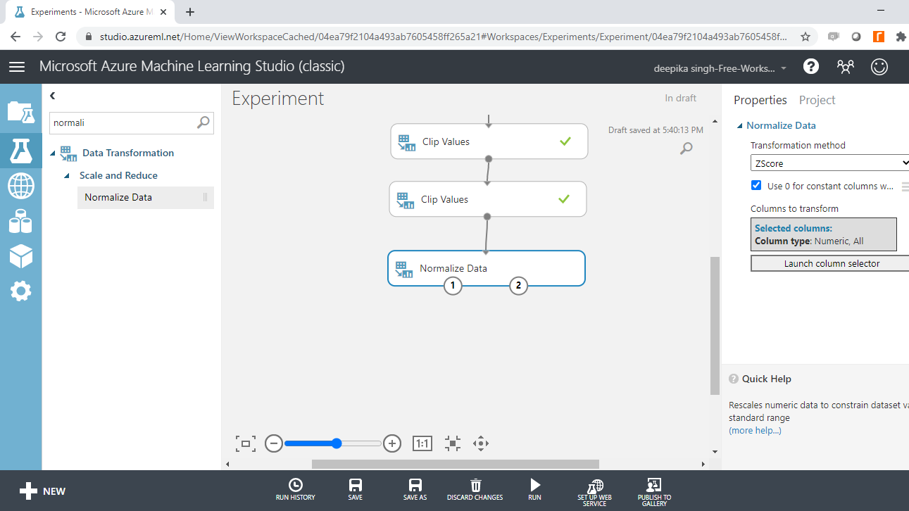
Click Launch column selector and select the variables.

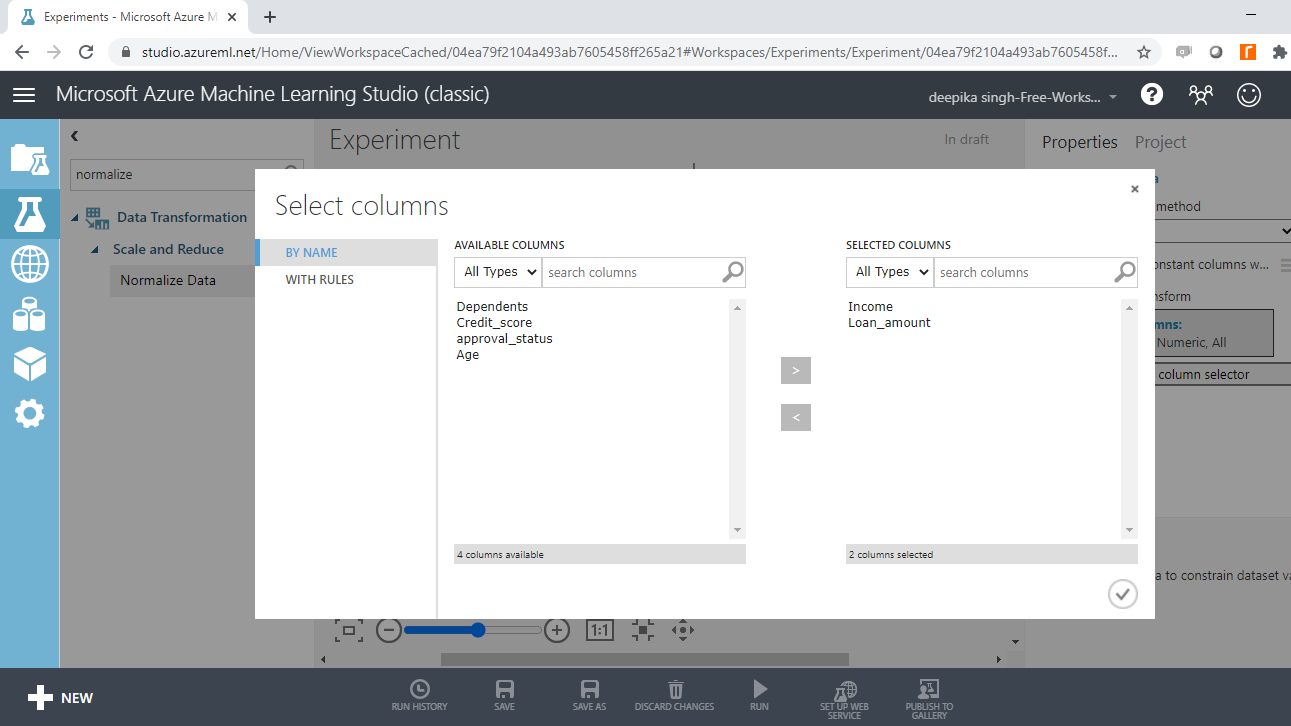
From the Transformation method dropdown list, choose the ZScore method to apply to all selected columns. A z-score measures how many standard deviations a data point is above or below the mean. The normalized variable takes a mean of zero and a standard deviation of one.

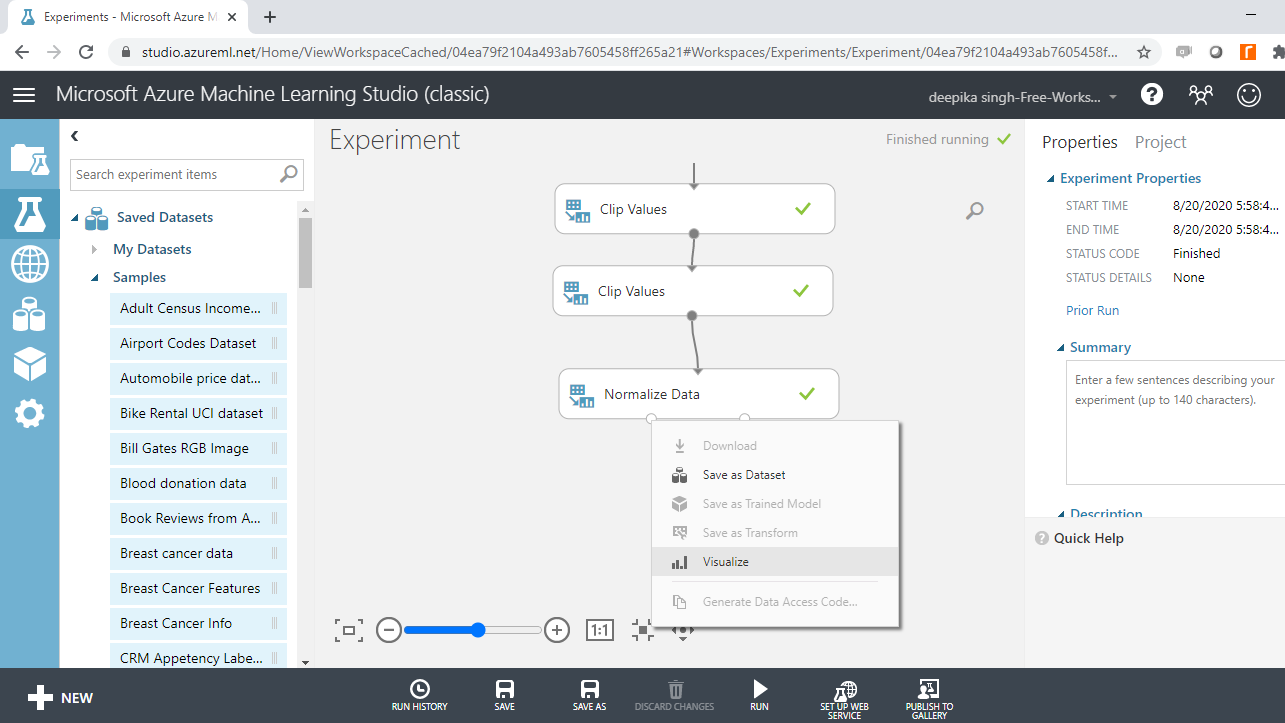
Click on Run. Next, right-click on the output port and select Visualize.

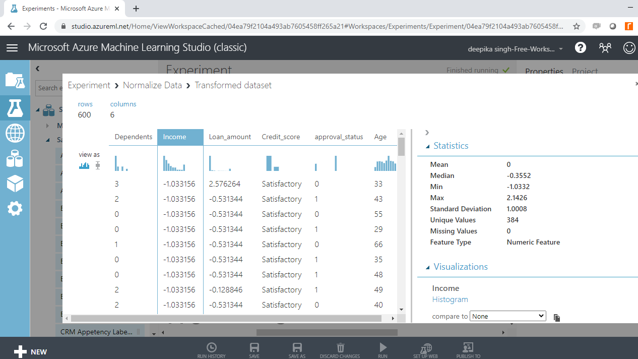
Selecting the Income variable will show that the variable has been normalized. It has a mean of zero and a standard deviation of one.

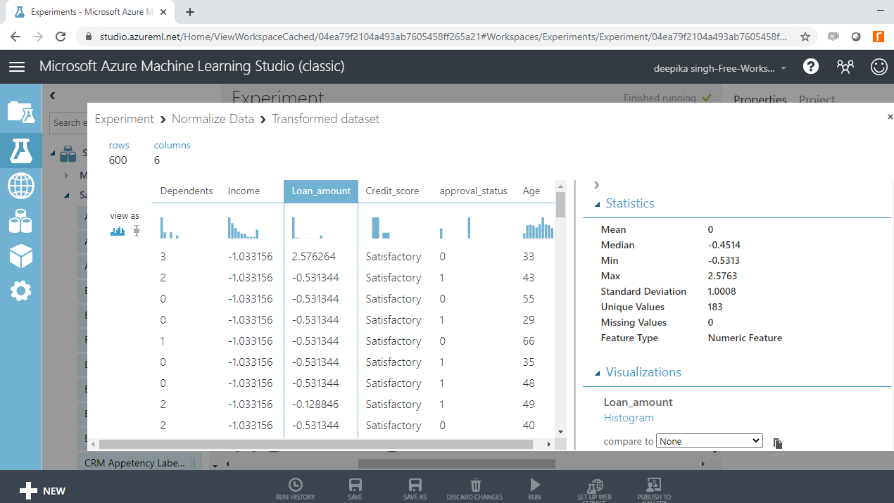
A similar result is obtained for the Loan_amount variable.

Binning or grouping data is another important tool in preparing numerical data for machine learning and is useful in scenarios when it is possible to convert a numeric feature into a categorical feature.

You can perform binning with the Group Data Into Bins module in Azure ML Studio. To try this, use the Age variable.

Next, search and drag the Group Data Into Bins module to your experiment.

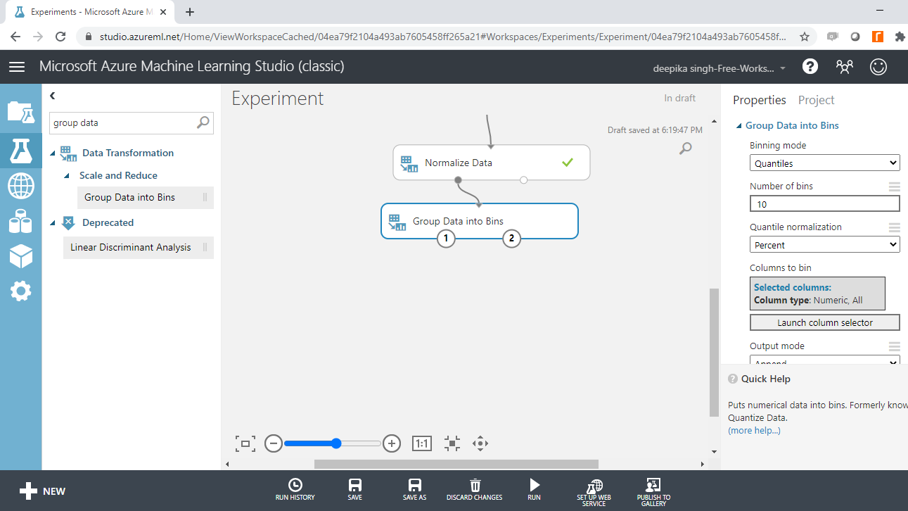
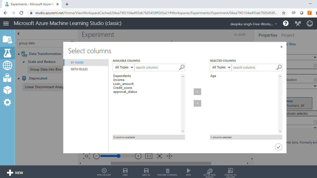
Next, click Launch column selector and select the Age variable.

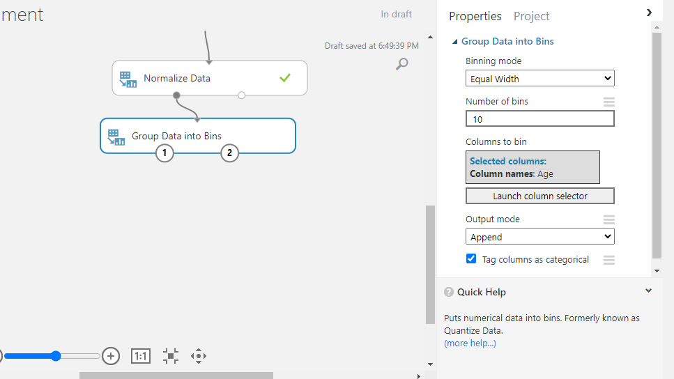
The next step is to set up the binning parameters. To start, select Equal width under Binning mode. This option requires specifying the number of bins, which is set to 10. In Equal width option, the values from the variable are placed in the bins such that each bin has the same interval between starting and end values. This results in some bins having more values than others if data is clumped around a certain point.

For Output mode, select the choice Append. This will create a new column with the binned values. Finally, select Tag columns as categorical to convert this new variable to a categorical feature.

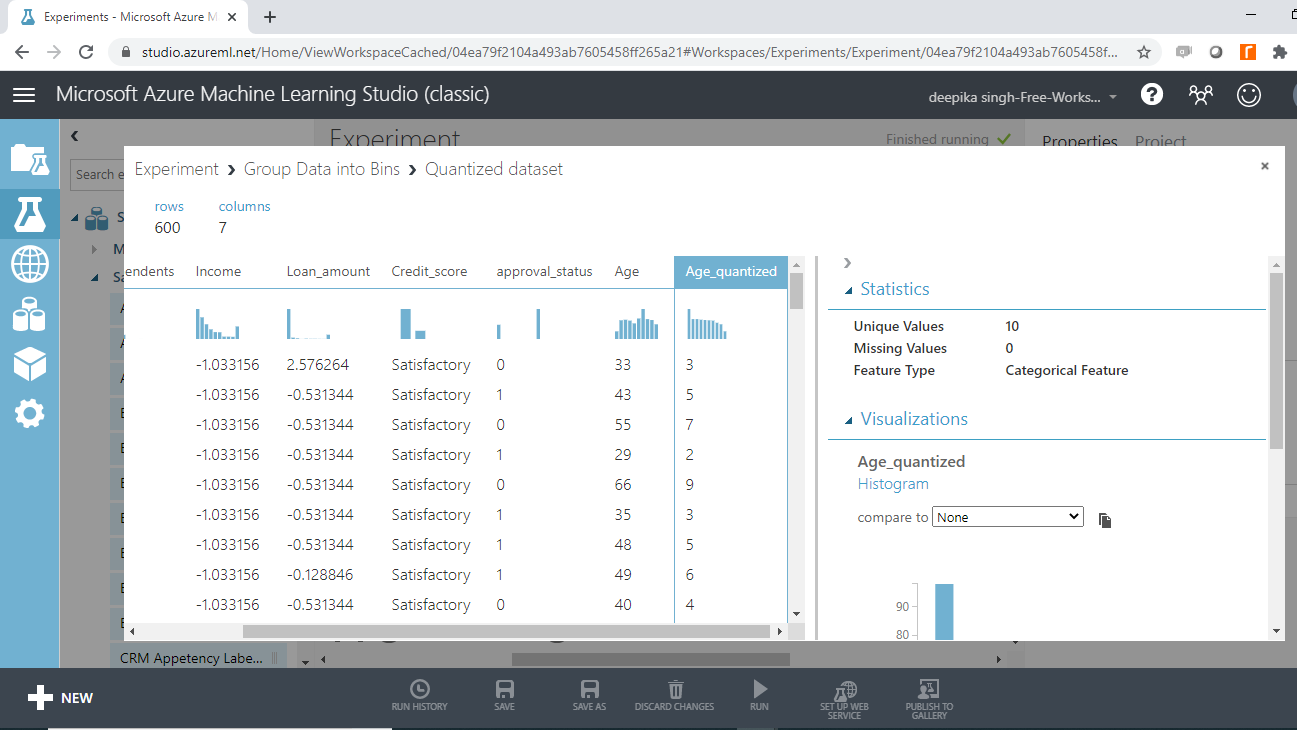
Run the experiment and from the output port of the Group Data into Bins module. Right-click and select the Visualize option as done previously to see the results.

The first result is the new quantized variable, Age_quantized, which is a categoric feature with ten unique values. These 10 unique values are the ten bins. The numbers one through ten in Age_quantized represent the bins to which that record belongs.

You can also look at the frequency distribution of total records in these bins by scrolling down in the workspace.

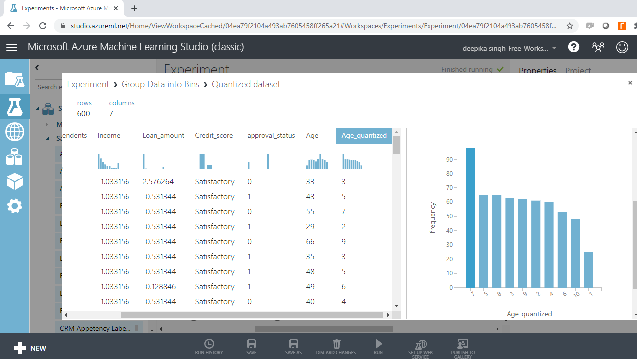
The above image shows that the bin with the highest number of records is the seventh bin, while the bin with the lowest number of records is the first bin.

In this guide, you learned how to perform common data preprocessing tasks with Azure ML Studio. You learned how to deal with incorrect entries, treat outliers, create bins for numerical variables, and normalize data in Azure ML Studio.

To learn more about data science and machine learning using Azure Machine Learning Studio, please refer to the following guides:

1. Getting Started with Azure ML Studio

2. Cleaning Data with Azure ML Studio