Getting Started with RNN
Sep 9, 2020 • 10 Minute Read
Introduction
Recurrent Neural Networks (RNNs) are a popular class of Artificial Neural Networks. RNNs are called recurrent because the output of each element of the sequence is dependent upon the previous computations.
When you watch a movie, you connect the dots because you know what happened in the last few scenes. Traditional NN architectures cannot do this. They cannot use previous scenes to predict what will happen in the next scene. Hence, to solve sequence-related problems, RNNs are used.
This tutorial will cover a brief introduction to simple RNNs and the concept of multi-layer perceptron (MLP). You will build a model on a time-series dataset to predict B value. Download the data here.
Understanding MLP
MLP is a feed-forward neural network. It consists of three nodes: an input layer, a hidden layer, and an output layer. They are fully connected as each node in one layer connects to a certain weight to every node in the following layer. MLP uses forward propagation followed by a supervised learning technique called backpropagation for training. A representation of MLP is shown below.
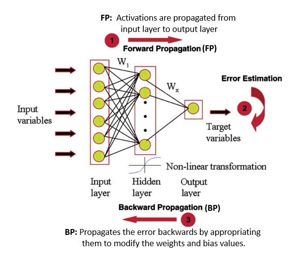
Image Source: Mashallah Rahimi
If you are interested in knowing more about backpropagation, refer to this blog post.
Understanding Simple RNNs
The idea behind an RNN is to make use of sequential information. The left side of the image below is a graphical illustration of the recurrence relation. The right part illustrates how the network unfolds through time over a sequence of length k. A typical unfolded RNN looks like this:
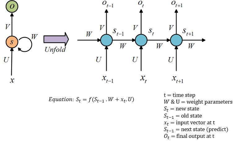
Image Source: researchgate.net
The optimal parameters for this task are U=W=1. Let's train the RNN model.
Understanding Backpropagation Through Time (BPTT) and Vanishing Gradient
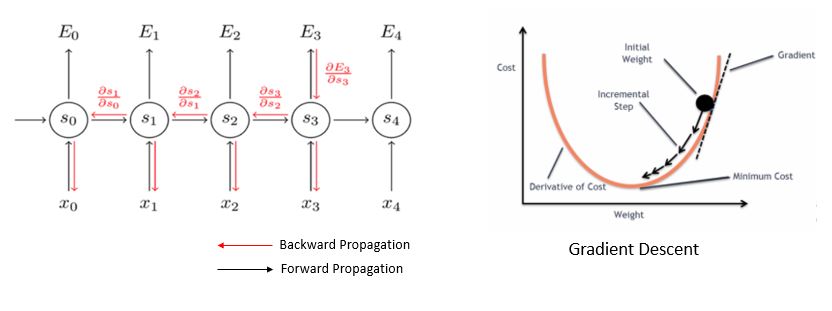
To train the RNNs, BPTT is used. "Through time" is appended to the term "backpropagation" to specify that the algorithm is being applied to a temporal neural model (RNN). The task of BPTT is to find a local minimum, a point with the least error. By adjusting the values of weights, the network can reach minima. This process is called gradient descent. Gradients (steps) are computed by derivatives, partial derivatives, and chain rule.
But BPTT has difficulty learning long-term dependencies. You might suggest adding more RNNs. Theoretically, that is correct, but practically, it's the opposite. Stacks of RNNs give rise to the vanishing gradient problem. BPTT would make the gradient so small, effectively preventing weights from changing its value, that it would completely stop the NN from training further.
Let's implement the code.
Code Implementation
You will be working with Bicton data, using 60 data points to predict the 61st data point.
      import numpy as np
import pandas as pd
import matplotlib.pyplot as plt
import warnings
from sklearn.metrics import mean_absolute_error
from keras.models import Sequential
from keras.layers import Dense, LSTM, Dropout,Flatten
warnings.filterwarnings("ignore")
Add a column for date and convert Timestamp columns to date form.
      bit_data=pd.read_csv("../input/bitstampUSD.csv")
bit_data["date"]=pd.to_datetime(bit_data["Timestamp"],unit="s").dt.date
group=bit_data.groupby("date")
data=group["Close"].mean()
data.shape
The goal is to make a prediction of daily close data. The last 60 rows are considered the test dataset.
      close_train=data.iloc[:len(data)-60]
close_test=data.iloc[len(close_train):]
Here values are set between 0-1 in order to avoid domination of high values.
      close_train=np.array(close_train)
close_train=close_train.reshape(close_train.shape[0],1)
from sklearn.preprocessing import MinMaxScaler
scaler=MinMaxScaler(feature_range=(0,1))
close_scaled=scaler.fit_transform(close_train)
Choose 60 data points as x-train and the 61st as y-train.
timestep=60
x_train=[]
y_train=[]
for i in range(timestep,close_scaled.shape[0]):
x_train.append(close_scaled[i-timestep:i,0])
y_train.append(close_scaled[i,0])
x_train,y_train=np.array(x_train),np.array(y_train)
x_train=x_train.reshape(x_train.shape[0],x_train.shape[1],1) #reshaped for RNN
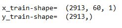
print("x-train-shape= ",x_train.shape)
print("y-train-shape= ",y_train.shape)
Implementation of MLP
The Keras sequential() API is used for creating the model. MLP is built on a stack of densely connected layers. Hence, the dense() function is added to extract important parameters. The first layer has 16 output neurons, and the next layer has eight outputs. Both are activated using ReLU.
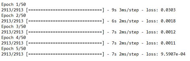
Next, compile the architecture by adjusting the hyperparameters. Here, optimizer is used for optimizing our model and loss function. Then, fit the training data to the model with 50 epochs, or iterations.
      model = Sequential()
model.add(Dense(56, input_shape=(x_train.shape[1],1), activation='relu'))
model.add(Dense(32, activation='relu'))
model.add(Flatten())
model.add(Dense(1)

model.compile(optimizer="adam",loss="mean_squared_error")
model.fit(x_train,y_train,epochs=50,batch_size=64)
Now the test data is been prepared for prediction.
      inputs=data[len(data)-len(close_test)-timestep:]
inputs=inputs.values.reshape(-1,1)
inputs=scaler.transform(inputs)
      x_test=[]
for i in range(timestep,inputs.shape[0]):
    x_test.append(inputs[i-timestep:i,0])
x_test=np.array(x_test)
x_test=x_test.reshape(x_test.shape[0],x_test.shape[1],1)
Let's apply the model on the test data.
      predicted_data=model.predict(x_test)
predicted_data=scaler.inverse_transform(predicted_data)
      data_test=np.array(close_test)
data_test=data_test.reshape(len(data_test),1)
Plot the predictions.
      plt.figure(figsize=(8,4), dpi=80, facecolor='w', edgecolor='k')
plt.plot(data_test,color="r",label="true result")
plt.plot(predicted_data,color="b",label="predicted result")
plt.legend()
plt.xlabel("Time(60 days)")
plt.ylabel("Values")
plt.grid(True)
plt.show()
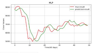
There is a huge gap between the true value and predicted results. The results aren't reliable. Let's implement RNN.
Implementation of Simple RNN
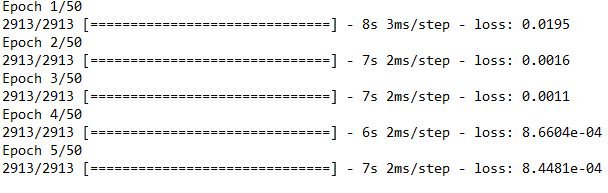
SimpleRNN will have a 2D tensor of shape (batch_size, internal_units) and an activation function of relu. As discussed earlier, RNN passes information through the hidden state, so let's keep true. A dropout layer is added after every layer. The matrix will be converted into one column using Flatten(). Lastly, compile the model.
      reg=Sequential()
reg.add(SimpleRNN(128,activation="relu",return_sequences=True,input_shape=(x_train.shape[1],1)))
reg.add(Dropout(0.25))
reg.add(SimpleRNN(256,activation="relu",return_sequences=True))
reg.add(Dropout(0.25))
reg.add(SimpleRNN(512,activation="relu",return_sequences=True))
reg.add(Dropout(0.35))
reg.add(Flatten())
reg.add(Dense(1))

reg.compile(optimizer="adam",loss="mean_squared_error")
reg.fit(x_train,y_train,epochs=50,batch_size=64)
it's time to predict.
      predicted_data=reg.predict(x_test)
predicted_data=scaler.inverse_transform(predicted_data)
      plt.figure(figsize=(8,4), dpi=80, facecolor='w', edgecolor='k')
plt.plot(data_test,color="r",label="true-result")
plt.plot(predicted_data,color="g",label="predicted-result")
plt.legend()
plt.xlabel("Time(60 days)")
plt.ylabel("Close Values")
plt.grid(True)
plt.show()
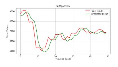
The results are still not satisfactory. This is due to the fading of the information (vanishing gradient). Read these additional guides on long short-term memory (LTSM) and gated recurrent units (GRU) to learn more about how they build on RNN and address this problem.
Conclusion
There is still a significant amount of lag between the outputs. There are several ways to address the vanishing gradient problem, one of which is gating. Gating decides when to forget the current input and when to remember it for future time steps. The most popular gating types today are LSTM and GRU.
You can try the above models with other data of your choice. I recommend changing some hyperparameter values and changing the number of layers and noting the difference in results.
Feel free to ask me any questions at Codealphabet.
Advance your tech skills today
Access courses on AI, cloud, data, security, and more—all led by industry experts.
