Getting Started with SAS for Machine Learning
Jul 16, 2020 • 8 Minute Read
Introduction
SAS is an enterprise-grade statistical software suite developed by SAS Institute. It is used for data management, advanced analytics, and predictive analytics, and has been one of the leading analytics platforms for a long time.
The SAS software contains all the necessary features required to design, develop, train, and evaluate machine learning models. In this guide, you will learn how to get started with SAS for machine learning.
SAS Studio Environment
To create a free subscription, visit this link. Once you have created your SAS profile, it will lead you to the landing page shown below.
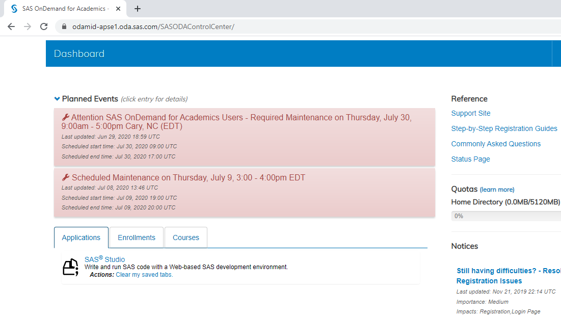
Click on the SAS Studio option under Applications, which will open the SAS Studio environment.
You are now ready to use SAS for machine learning.
Loading Data
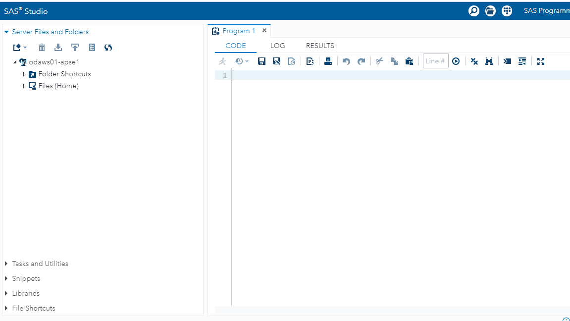
In the above image, there are many features of SAS Studio listed on the left sidebar, such as Server Files and Folders, Tasks and Utilities, Snippets, etc.
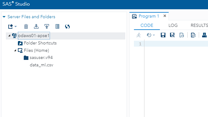
To import data from your local system, click on the upload symbol under Server Files and Folders.
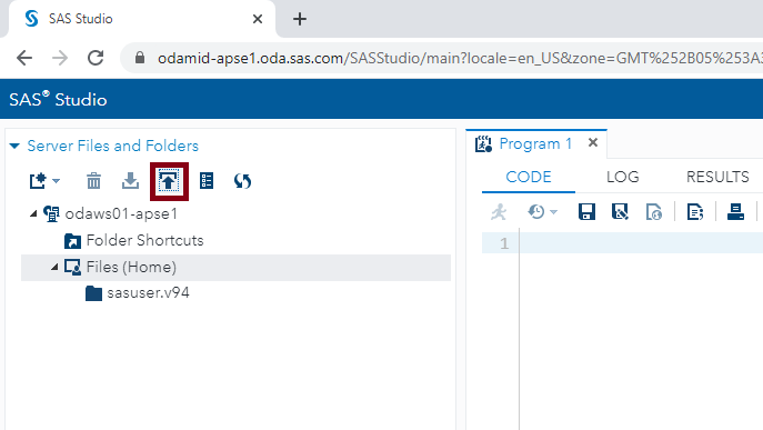
The above selection will open a tab for importing data from the local system. Once this step is completed, the data will appear in the pane.
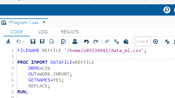
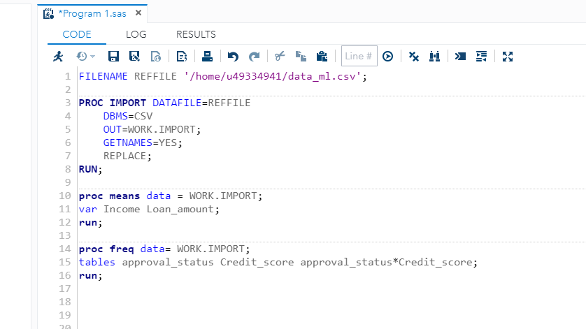
You now have data in SAS Studio, and the next step is to bring it into the CODE pane. This is done with the code below, which uses the PROC IMPORT statement to import the data into the coding environment.
PROC is a group of SAS procedure statements to identify and analyze the data in SAS. You can also perform graphics and variable operations with PROC.
The first line of code below tells SAS where the file to import is stored and what the file name is. The DBMS option indicates that you are importing a CSV file. The OUT command names the output dataset for further use.
Finally, the REPLACE option informs SAS that it is permissible to overwrite the dataset created to re-run the exact same PROC IMPORT code in the future if needed.
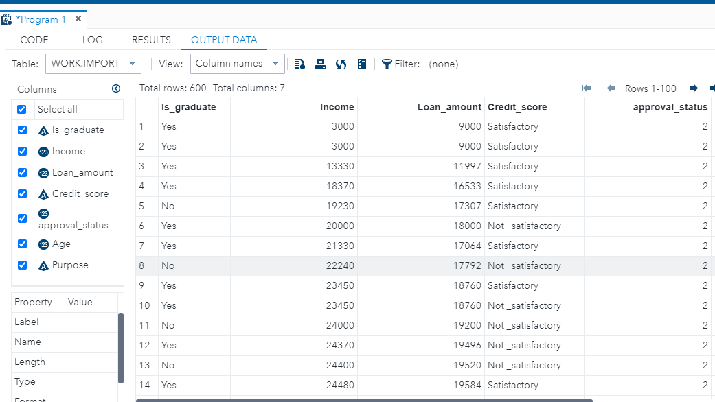
Once you have executed the code, it will generate a display in the new OUTPUT DATA tab, as shown below.
Understanding the Data
For this example, I have imported a fictitious dataset of loan applicants containing 600 observations and seven variables, as described below:
-
Is_graduate: Whether the applicant is a graduate ("Yes") or not ("No")
-
Income: Annual Income of the applicant (in USD)
-
Loan_amount: Loan amount (in USD) for which the application was submitted
-
Credit_score: Whether the applicant's credit score is satisfactory or not.
-
Approval_status: Whether the loan application was approved ("1") or not ("2")
-
Age: The applicant's age in years
-
Purpose: Purpose of applying for the loan
Exploring Features
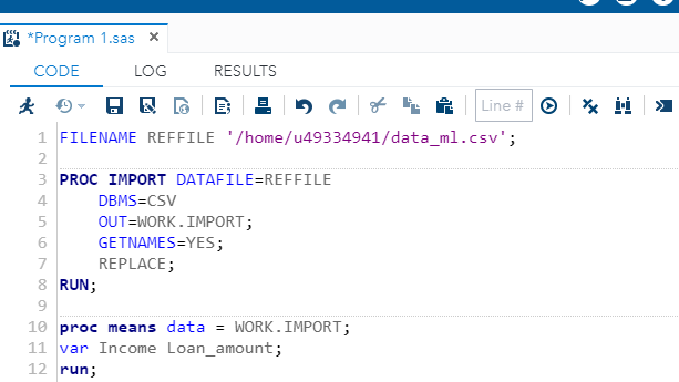
You can explore numerical and categorical variables in SAS. To calculate summary statistics of the quantitative variables, you can use the proc means command. This is shown in lines 10 to 12 below. The run command tells SAS that you want to execute the specified lines of code.
Run the above command to generate the following output.
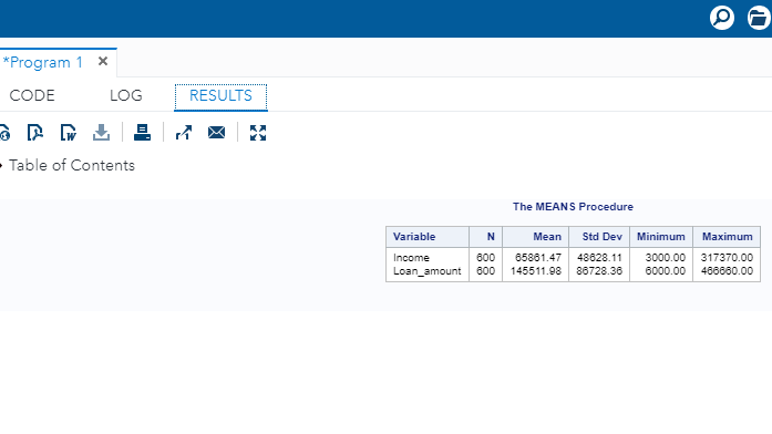
The output above shows the basic statistics for the variables Income and Loan_amount. There are 600 observations, equivalent to the total record in the dataset, which indicates no missing values for these two variables. Also, the average income of the applicants is $65,861, while the mean loan amount applied for is $145,511.
You can also explore the categorical variables with the proc freq command. The code displayed in lines 14 to 16, looks at the frequency cross tabulation of two important categorical variables, approval_status and Credit_score.
The above command will generate the following output.
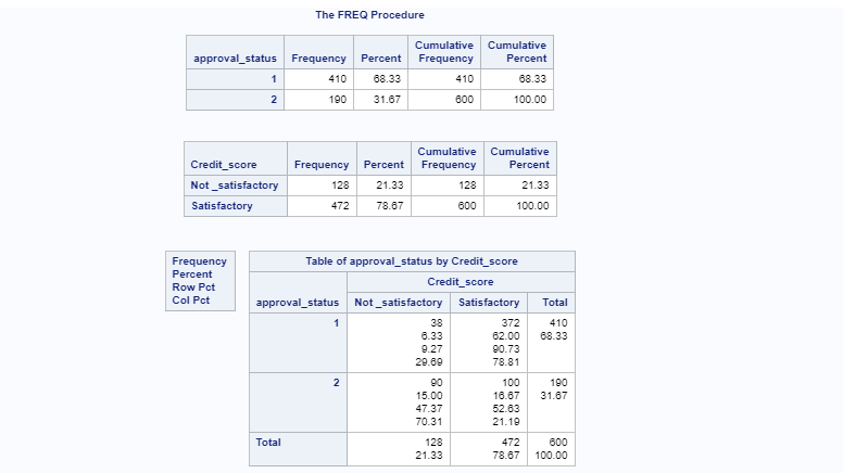
The above output shows the frequency distribution of labels for approval_status and Credit_score. The cross tabulation shows the intersection between these variables. For approved loan applicants, indicated by the approval status label 1, the credit score was satisfactory in 90.73% of cases. This indicates that credit score is a strong predictor of loan approval.
Building the Model
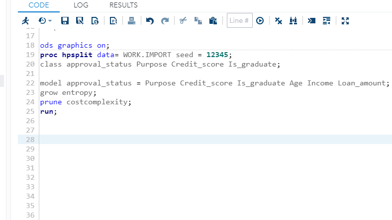
You will now learn how to build a decision tree model with the HPSPLIT procedure in SAS studio. The HPSPLIT procedure provides commands that build tree-based statistical models for classification and regression. Both are referred to as decision trees because the model is expressed as a series of if-then statements.
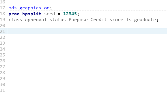
Start with the code below. The first line turns ods graphics on. ODS stands for output delivery system and manages the output and its display. The second line uses the proc hpsplit command and sets the random seed for reproducibility. Next, you will specify the categorical variables of the data with the class statement.
The next step is to write the model equation, which is done in lines 22 to 25 below. The model building starts with the model command, which contains the target variable, approval_status, and all the other variables separated by an equal sign.
The grow and prune statements control two fundamental aspects of building decision trees—growing and pruning.
In the code below, use the grow statement to specify the criterion for splitting internal nodes into additional sub-nodes or terminal nodes. These are also referred to as parent and child nodes as the tree is grown.
The HPSPLIT procedure provides different types of criteria for growing a full decision tree that minimizes the nodes' impurity or error. One such criterion is entropy, which is specified in the code.
Another important command in the code is prune costcomplexity. A decision tree often overfits the training data, leading to generalization error on validation or test data. The solution is to find a smaller subtree with the prune statement. The most common pruning method is through cost complexity, which makes a trade-off between the tree size and the error rate to help prevent over-fitting. The last step is to run the command after specifying the model building choices.
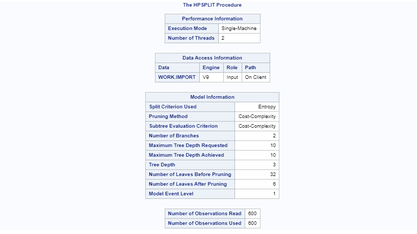
Executing the run command above will display the output in the RESULTS tab of SAS Studio. The first major output prints the summary of the model procedure. It explains parameters like the split criterion, number of leaves before and after pruning, and other details.
The other major output is the confusion matrix used to evaluate model performance.
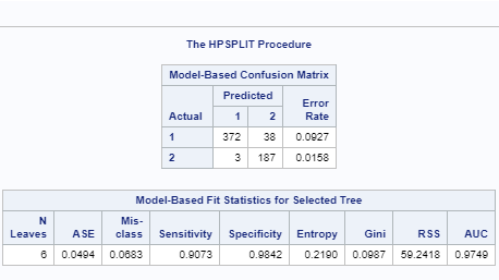
The confusion matrix and the table above show that the sensitivity, specificity, and accuracy of the model are 90.7%, 98.4%, and 93.2%, respectively. These are impressive numbers that indicate that the model is performing well.
Conclusion
In this guide, you got started with the popular and powerful statistical software SAS. You learned how to create a free account and load data into the workspace. You also learned how to explore, build, and evaluate the classification algorithm. This will get you started in building machine learning models with SAS.
Advance your tech skills today
Access courses on AI, cloud, data, security, and more—all led by industry experts.
