Artistic Neural Style Transfer with TensorFlow 2.0, Part 2: Implementation
Jun 3, 2020 • 13 Minute Read
Introduction
This is the second guide in a two-part series on artistic neural style transfer. Part 1 walked through separating the convolution layer for style and content images to extract their respective features. When the loss function is tuned, it combines these features to generate a styled image. This guide, Part 2, will go deeper into style loss and content loss.
Usually, in deep learning, we have only one loss function. However, in neural style transfer, we are generating a new image from two images, so we need more loss functions to generate a new image. We will discuss various loss functions such as content loss, style loss, and variation loss.
There are many approaches to mathematical notation. The equations in this guide are taken from Gatsy et al. (some notations might differ).
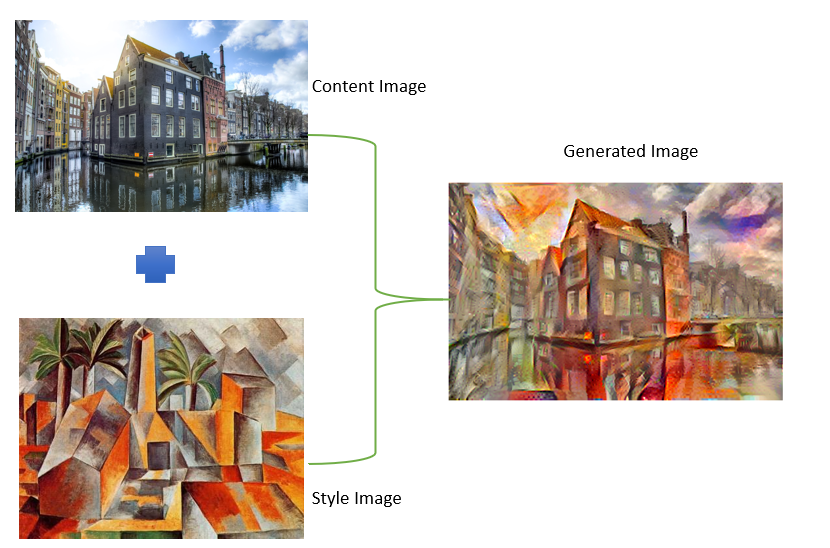
Below is a simple representation of how the new image will be generated from the content and style images.
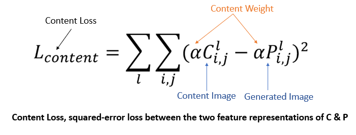
Content Loss
This function helps to check how similar the generated image is to the content image. It gives the measure of how far (different) are the features of the content image and target image. The Euclidean distance is calculated. It is defined as follows:
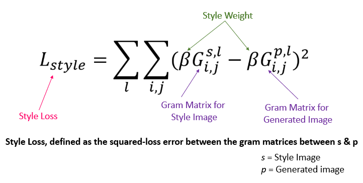
Style Loss
Style Loss measures how different the generated image, in terms of style features, is from your style image. But it's not as straightforward as content loss. The style representation of an image is given by Gram Matrix.
Gram Matrix
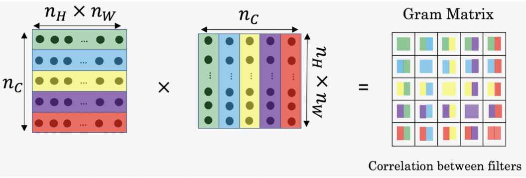
Gram Matrix is only concerned with whether the stylish features are present in image weights, textures, and shapes. Hence, it is the best choice. The Gram Matrix G is the set of vectors in a matrix of dot products. For a particular layer, the diagonal elements of the matrix will find how active the filter is. An active filter will help the model find wether it contains more horizontal lines, vertical lines, or textures.
To get the results, the matrix is multiplied by its transposed matrix.
Its equation is as follows:
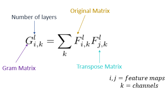
The GM helps you find how similar Fik is to Fjk. If the dot product is large, they are highly similar.
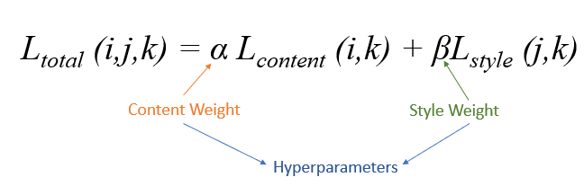
Finally, total loss will minimize the weighted average.
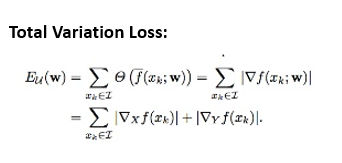
Variation Loss
Variation loss was introduced to avoid highly noisy outputs and overly pixelated results. The main purpose of variation loss is to maintain smoothness and spatial continuity.
The change in the combination of images minimizes the loss so that you can have an image combination of both the Picasso painting and the input image. To make the losses bit smaller, an optimization algorithm is used. The first order algorithm uses a gradient to minimize the loss function, famously known as gradient descent. The Adam optimization shows faster results in style transfer.
Code Implementation
In this section, we will implement the code to generate a Gram Matrix from the input image tensor and the model that will generate the image.
GM can be implemented concisely using the tf.linalg.einsum function:
      def gram_matrix(input_tensor):
  result = tf.linalg.einsum('bijc,bijd->bcd', input_tensor, input_tensor)
  input_shape = tf.shape(input_tensor)
  num_locations = tf.cast(input_shape[1]*input_shape[2], tf.float32)
  return result/(num_locations)
Build a model that returns the style and content tensors.
      class StyleContentModel(tf.keras.models.Model):
  def __init__(self, style_layers, content_layers):
    super(StyleContentModel, self).__init__()
    self.vgg =  vgg_layers(style_layers + content_layers)
    self.style_layers = style_layers
    self.content_layers = content_layers
    self.num_style_layers = len(style_layers)
    self.vgg.trainable = False

  def call(self, inputs):
    "Expects float input in [0,1]"
    inputs = inputs*255.0
    preprocessed_input = tf.keras.applications.vgg19.preprocess_input(inputs)
    outputs = self.vgg(preprocessed_input)
    style_outputs, content_outputs = (outputs[:self.num_style_layers],
                                      outputs[self.num_style_layers:])

    style_outputs = [gram_matrix(style_output)
                     for style_output in style_outputs]

    content_dict = {content_name:value
                    for content_name, value
                    in zip(self.content_layers, content_outputs)}

    style_dict = {style_name:value
                  for style_name, value
                  in zip(self.style_layers, style_outputs)}

    return {'content':content_dict, 'style':style_dict}
When called on an image, this model returns the gram matrix (style) of the style_layers and content of the content_layers:
      extractor = StyleContentModel(style_layers, content_layers)

results = extractor(tf.constant(content_image))

print('Styles:')
for name, output in sorted(results['style'].items()):
  print("  ", name)
  print("    shape: ", output.numpy().shape)
  print("    min: ", output.numpy().min())
  print("    max: ", output.numpy().max())
  print("    mean: ", output.numpy().mean())
  print()

print("Contents:")
for name, output in sorted(results['content'].items()):
  print("  ", name)
  print("    shape: ", output.numpy().shape)
  print("    min: ", output.numpy().min())
  print("    max: ", output.numpy().max())
  print("    mean: ", output.numpy().mean())

Set your style and content target values and run gradient descent:
      style_targets = extractor(style_image)['style']
content_targets = extractor(content_image)['content']
The tf.variables are used to assign biases and weights throughout the training session. These weights are then used for optimization. They are initialized with the content image.
Note: tf.variable and the content image are the same size.
image = tf.Variable(content_image)
Since this is a float image, define a function to keep the pixel values between 0 and 1:
      def clip_0_1(image):
  return tf.clip_by_value(image, clip_value_min=0.0, clip_value_max=1.0)
Set the variables for the Adam optimizer.
opt = tf.optimizers.Adam(learning_rate=0.02, beta_1=0.99, epsilon=1e-1)
Get the total loss use the weighted combination of style and content losses.
      style_weight=1e-2
content_weight=1e4
Now comes the main part: loss function!
      def style_content_loss(outputs):
    style_outputs = outputs['style']
    content_outputs = outputs['content']
    style_loss = tf.add_n([tf.reduce_mean((style_outputs[name]-style_targets[name])**2)
                           for name in style_outputs.keys()])
    style_loss *= style_weight / num_style_layers

    content_loss = tf.add_n([tf.reduce_mean((content_outputs[name]-content_targets[name])**2)
                             for name in content_outputs.keys()])
    content_loss *= content_weight / num_content_layers
    loss = style_loss + content_loss
    return loss
The tf.function will speed up the operation. Defining train_step will send the gradient to the optimizer. tf.GradientTape() calculates the gradients of the function based on its composition automatically.
      @tf.function()
def train_step(image):
  with tf.GradientTape() as tape:
    outputs = extractor(image)
    loss = style_content_loss(outputs)

  grad = tape.gradient(loss, image)
  opt.apply_gradients([(grad, image)])
  image.assign(clip_0_1(image))
Now run a few steps to test:
      train_step(image)
train_step(image)
train_step(image)
tensor_to_image(image)
import time
start = time.time()
epochs = 10
steps_per_epoch = 100
step = 0
for n in range(epochs):
for m in range(steps_per_epoch):
step += 1
train_step(image)
print(".", end='')
display.clear_output(wait=True)
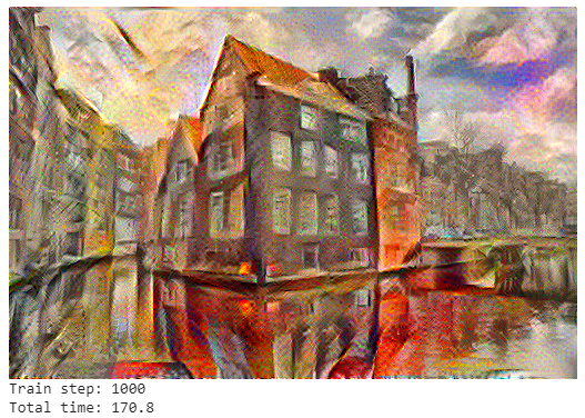
display.display(tensor_to_image(image))
print("Train step: {}".format(step))
end = time.time()
print("Total time: {:.1f}".format(end-start))
Now add total variation loss to reduce the high frequency artifacts. Apply high frequency explicit regularization term on the high frequency components of the image. The difference between the neighboring pixels is shown below:
      def high_pass_x_y(image):
  x_var = image[:,:,1:,:] - image[:,:,:-1,:]
  y_var = image[:,1:,:,:] - image[:,:-1,:,:]

  return x_var, y_var
The comparison of horizontal (width) and vertical (height) high-frequency components (edge-detection) for content of a styled image is shown below.
      x_deltas, y_deltas = high_pass_x_y(content_image)

plt.figure(figsize=(14,10))
plt.subplot(2,2,1)
imshow(clip_0_1(2*y_deltas+0.5), "Horizontal Deltas: Original")

plt.subplot(2,2,2)
imshow(clip_0_1(2*x_deltas+0.5), "Vertical Deltas: Original")

x_deltas, y_deltas = high_pass_x_y(image)

plt.subplot(2,2,3)
imshow(clip_0_1(2*y_deltas+0.5), "Horizontal Deltas: Styled")

plt.subplot(2,2,4)
imshow(clip_0_1(2*x_deltas+0.5), "Vertical Deltas: Styled")
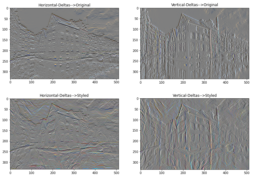
This shows how the high-frequency components have increased.
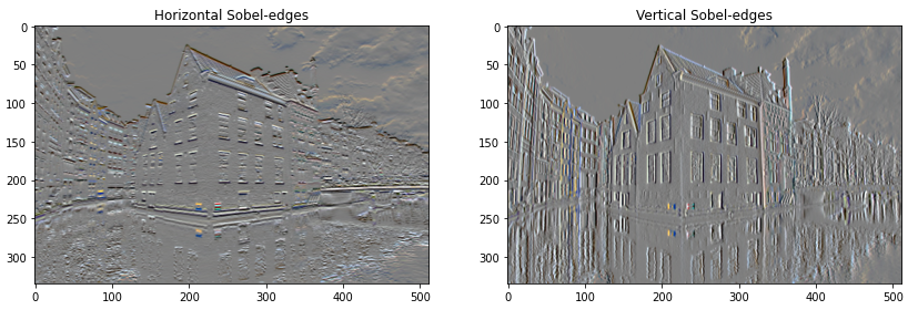
You can get similar output from the Sobel edge detector, for example:
      plt.figure(figsize=(14,10))

sobel = tf.image.sobel_edges(content_image)
plt.subplot(1,2,1)
imshow(clip_0_1(sobel[...,0]/4+0.5), "Horizontal Sobel-edges")
plt.subplot(1,2,2)
imshow(clip_0_1(sobel[...,1]/4+0.5), "Vertical Sobel-edges")
Optimize the squared value by finding the rate of change of edges with high_pass_x_y.
      def total_variation_loss(image):
  x_deltas, y_deltas = high_pass_x_y(image)
  return tf.reduce_sum(tf.abs(x_deltas)) + tf.reduce_sum(tf.abs(y_deltas))
total_variation_loss(image).numpy()
Output: 89581.1
tf.image.total_variation(image).numpy()
array([89581.1], dtype=float32)
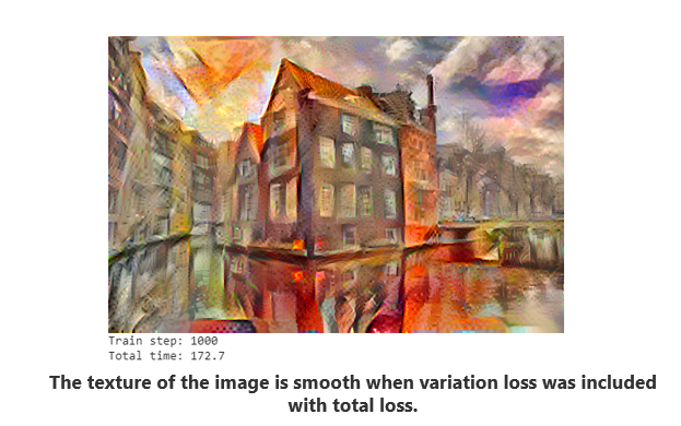
Re-run the optimization and adjust total variation weight.
total_variation_weight=30
      @tf.function()
def train_step(image):
  with tf.GradientTape() as tape:
    outputs = extractor(image)
    loss = style_content_loss(outputs)
    loss += total_variation_weight*tf.image.total_variation(image)

  grad = tape.gradient(loss, image)
  opt.apply_gradients([(grad, image)])
  image.assign(clip_0_1(image))
image = tf.Variable(content_image)
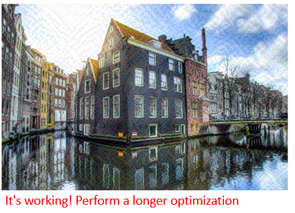
Call the overall method. Notice the change in patterns after every 100 epochs.
      import time
start = time.time()

epochs = 10
steps_per_epoch = 100

step = 0
for n in range(epochs):
  for m in range(steps_per_epoch):
    step += 1
    train_step(image)
    print(".", end='')
  display.clear_output(wait=True)
  display.display(tensor_to_image(image))
  print("Train step: {}".format(step))

end = time.time()
print("Total time: {:.1f}".format(end-start))
Save the results.
Conclusion
Congratulations! You are the owner of unique, amazing digital art. You can now play with different images and paintings to adjust the weights of style and content features and see the changes. I also recommend reading this blog to gain in-depth knowledge of gradient descent.
This guide also contains many mathematical equations, and I recommend reading the paper mentioned above to understand their purpose. Knowing the purpose will help you modify them if required.
This whole implementation is done in Tensorflow 2.0. When you run it, you'll notice that it is much slower even on GPUs. In a future guide, we will look at how to implement a shorter and faster version of the same functionality in PyTorch.
To learn more about this topic or other machine learning solutions, feel free to contact me here.