Polynomial Functions Analysis with R
Aug 24, 2020 • 7 Minute Read
Introduction
When you have feature points aligned in almost a straight line, you can use simple linear regression or multiple linear regression (in the case of multiple feature points). But how will you fit a function on a feature(s) whose points are non-linear? In this guide you will learn to implement polynomial functions that are suitable for non-linear points. You will be working in R and should already have a basic knowledge on regression to follow along.
Describing the Original Data and Creating Train and Test Data
Original Data
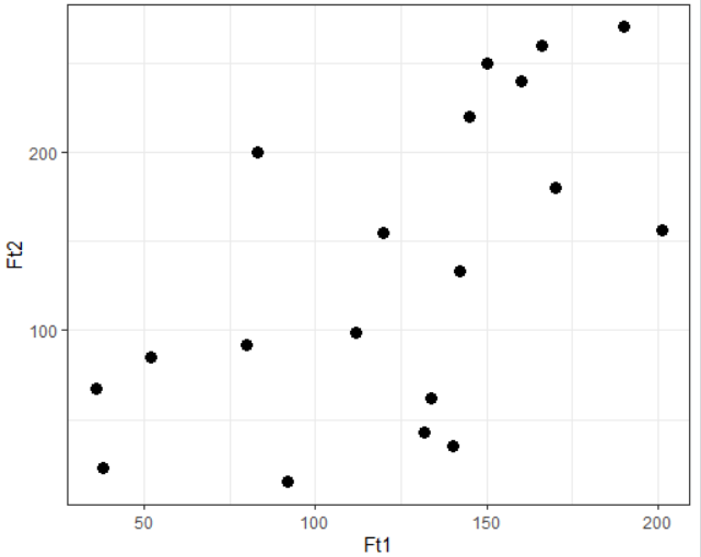
Consider a dependent variable Ft1 and an independent variable Ft2 with 19 data points as shown:
| Ft1 | Ft2 |
|---|---|
| 38 | 23 |
| 52 | 85 |
| 36 | 67 |
| 92 | 15 |
| 83 | 200 |
| 170 | 180 |
| 140 | 35 |
| 201 | 156 |
| 112 | 99 |
| 132 | 43 |
| 80 | 92 |
| 134 | 62 |
| 150 | 250 |
| 160 | 240 |
| 190 | 270 |
| 145 | 220 |
| 166 | 260 |
| 120 | 155 |
| 142 | 133 |
You can visualize the complete data using the ggplot2 library as shown:
      # Load ggplot2 library
library(ggplot2)

# Load data from a CSV file
data <- read.csv("file.csv")

# Visualize the data
ggplot(data) +
  geom_point(aes(Ft1, Ft2),size=3) +
  theme_bw()
Creating Train and Test Data
You can split the original data into train and test in a ratio of 75:25 with the following code:
      # Set a seed value for reproducible results
set.seed(70)

# Split the data
ind <- sample(x = nrow(data), size = floor(0.75 * nrow(data)))

# Store the value in train and test dataframes
train <- data[ind,]
test <- data[-ind,]
Building Polynomial Regression of Different Degrees
To build a polynomial regression in R, start with the lm function and adjust the formula parameter value. You must know that the "degree" of a polynomial function must be less than the number of unique points.
At this point, you have only 14 data points in the train dataframe, therefore the maximum polynomial degree that you can have is 13. The given code builds four polynomial functions of degree 1, 3, 5, and 9.
      # Order 1
poly_reg1 <- lm(formula = Ft1~poly(Ft2,1),
                data = train)
# Order 3
poly_reg3 <- lm(formula = Ft1~poly(Ft2,3),
                data = train)
# Order 5
poly_reg5 <- lm(formula = Ft1~poly(Ft2,5),
                data = train)
# Order 9
poly_reg9 <- lm(formula = Ft1~poly(Ft2,9),
                data = train)
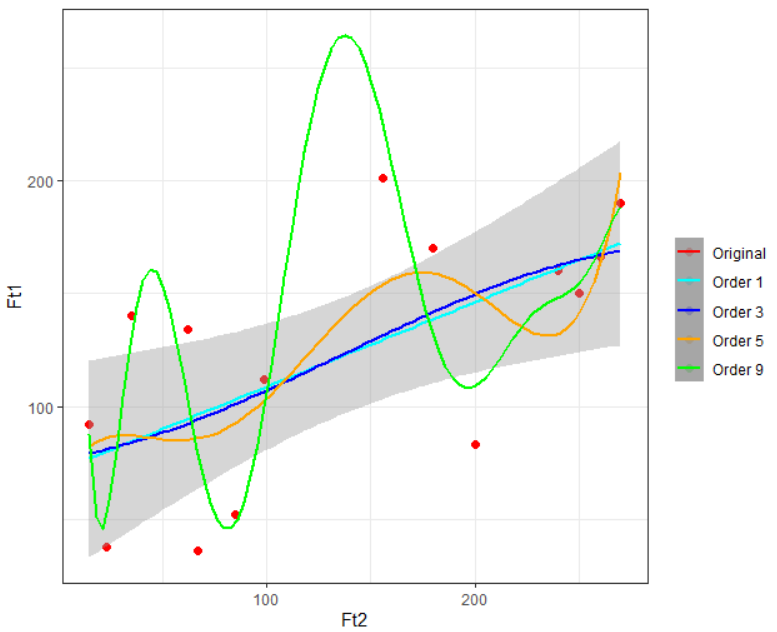
Once you have successfully built these four models you can visualize them on your training data using the given ggplot code:
      ggplot(train) +
  geom_point(aes(Ft2, Ft1, col = "Original"), cex = 2) +
  stat_smooth(method = "lm", formula = y~poly(x,1), aes(Ft2, poly_reg1$fitted.values, col = "Order 1")) +
  stat_smooth(method = "lm", formula = y~poly(x,3), aes(Ft2, poly_reg3$fitted.values, col = "Order 3")) +
  stat_smooth(method = "lm", formula = y~poly(x,5), aes(Ft2, poly_reg5$fitted.values, col = "Order 5")) +
  stat_smooth(method = "lm", formula = y~poly(x,9), aes(Ft2, poly_reg9$fitted.values, col = "Order 9")) +
  scale_colour_manual("",
                      breaks = c("Original",  "Order 1", "Order 3", "Order 5", "Order 9"),
                      values = c("red","cyan", "blue","orange","green")) +
  theme_bw()
Measuring the RSS Value on Train and Test Data
You have all the information to get the RSS value on train data, but to get the RSS value of test data, you need to predict the Ft1 values. Use the given code to do so:
      # Predicting values using test data by each model
poly1_pred <- predict(object = poly_reg1,
                      newdata =  data.frame(Ft2 = test$Ft2))
poly3_pred <- predict(object = poly_reg3,
                      newdata =  data.frame(Ft2 = test$Ft2))
poly5_pred <- predict(object = poly_reg5,
                      newdata =  data.frame(Ft2 = test$Ft2))
poly9_pred <- predict(object = poly_reg9,
                      newdata =  data.frame(Ft2 = test$Ft2))
Now, you can find RSS values for both the data as shown:
      # RSS for train data based on each model
train_rss1 <- mean((train$Ft1 - poly_reg1$fitted.values)^2)  # Order 1
train_rss3 <- mean((train$Ft1 - poly_reg3$fitted.values)^2)  # Order 3
train_rss5 <- mean((train$Ft1 - poly_reg5$fitted.values)^2)  # Order 5
train_rss9 <- mean((train$Ft1 - poly_reg9$fitted.values)^2)  # Order 9

# RSS for test data based on each model
test_rss1 <- mean((test$Ft1 - poly1_pred)^2)  # Order 1
test_rss3 <- mean((test$Ft1 - poly3_pred)^2)  # Order 3
test_rss5 <- mean((test$Ft1 - poly5_pred)^2)  # Order 5
test_rss9 <- mean((test$Ft1 - poly9_pred)^2)  # Order 9
| train_rss1 | train_rss3 | train_rss5 | train_rss9 |
|---|---|---|---|
| 0.000 | 1673.867 | 1405.703 | 436.5995 |
| test_rss1 | test_rss3 | test_rss5 | test_rss9 |
|---|---|---|---|
| 42004.6972 | 669.9034 | 725.9172 | 5385.6354 |
From the above two tables you can observe that the RSS value for train data starts to decrease after the first degree, which means the higher the degree better the curve fitting and reduced error. However, at the same time the test RSS increases with the increase of the degree, which implies underfitting. You can observe these patterns from the given plot.
      # Visualizing train and test RSS for each model

# excluding degree 1
train_rss <- scale(c(train_rss3, train_rss5, train_rss9)) # scaling
test_rss <- scale(c(test_rss3, test_rss5, test_rss9))      # scaling
orders <- c(3, 5, 9)

ggplot() +
  geom_line(aes(orders, train_rss, col = "Train RSS")) +
  geom_line(aes(orders, test_rss, col = "Test RSS")) +
  scale_colour_manual("",
                      breaks = c("Train RSS", "Test RSS"),
                      values = c("green", "red")) +
  theme_bw() + ylab("RSS")
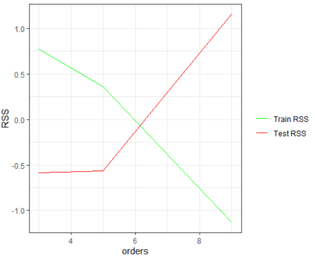
From this plot you can deliver an insight that only the polynomial of degree five is optimal for this data, as it will give the lowest error for both the train and the test data.
Conclusion
You have learned to apply polynomial functions of various degrees in R. You observed how underfitting and overfitting can occur in a polynomial model and how to find an optimal polynomial degree function to reduce error for both train and test data.
Advance your tech skills today
Access courses on AI, cloud, data, security, and more—all led by industry experts.
