Troubleshooting Excel Formulas
Jun 3, 2020 • 7 Minute Read
Introduction
If you are an Excel user, you may have been writing Excel formulas from day one, or you may just be learning how helpful they can be. Either way, it's likely that you run into problems from time to time. Just like any other programming language or statistical tool, Excel provides a way to decompose a formula, however long it may be, and perform step-by-step calculations. This way, you can jump inside a nested formula and understand how it works.
In this guide, you will learn to troubleshoot Excel formulas by walking through a scenario based on calculating the distance between two coordinate points and then normalizing the resulted distance. You'll need to understand operator precedence for this guide. For a quick review, you can refer to Wikipedia: Order of operations.
Set Up the Data
Consider this table, which consists of five rows each with two coordinate points (x,y):
| X1 | Y1 | X2 | Y2 |
|---|---|---|---|
| -1 | 8 | 16 | 32 |
| -8 | 789.8 | 2 | 8 |
| 13.45 | -0.2 | 63 | -4 |
| -4 | -8000 | 130 | -7 |
| -7 | -8 | 9 | 150 |
First, calculate the Euclidean distance, or shortest distance, between each of the pairs. The Euclidean distance is represented as:
d = sqrt( (x2 - x1)^2 + (y2 - y1)^2 )
Create a new column named Euclidean Distance and use the formula above to arrive at the following table:
| X1 | Y1 | X2 | Y2 | Euclidean Distance |
|---|---|---|---|---|
| -1 | 8 | 16 | 32 | 29.41088234 |
| -8 | 789.8 | 2 | 8 | 781.8639524 |
| 13.45 | -0.2 | 63 | -4 | 49.69549778 |
| -4 | -8000 | 130 | -7 | 7994.123154 |
| -7 | -8 | 9 | 150 | 158.8080602 |
Notice that the resulting Euclidean Distance column values are not rounded up and they are spread across a range [29.4, 7994.1].
The next step is to normalize the distance values in a range [0, 1] using the given formula:
x_current = (x_current - x_minimum) / (x_maximum - x_minimum)
By applying the above formula to the Euclidean Distance column values, you get this table:
| X1 | Y1 | X2 | Y2 | Euclidean Distance | Normalized Euclidean Distance |
|---|---|---|---|---|---|
| -1 | 8 | 16 | 32 | 29.41088234 | 0 |
| -8 | 789.8 | 2 | 8 | 781.8639524 | 0.094473353 |
| 13.45 | -0.2 | 63 | -4 | 49.69549778 | 0.002546811 |
| -4 | -8000 | 130 | -7 | 7994.123154 | 1 |
| -7 | -8 | 9 | 150 | 158.8080602 | 0.016246309 |
Notice that all the values in the Normalized Euclidean Distance column lie in a range of [0, 1]. With the data setup completed, let's learn how Excel computes these formula outputs step by step.
Access the Evaluate Formula Tool
To troubleshoot any Excel formula, follow these steps:
- Select an appropriate cell to evaluate from a column (don't select a range of cells or the complete column)
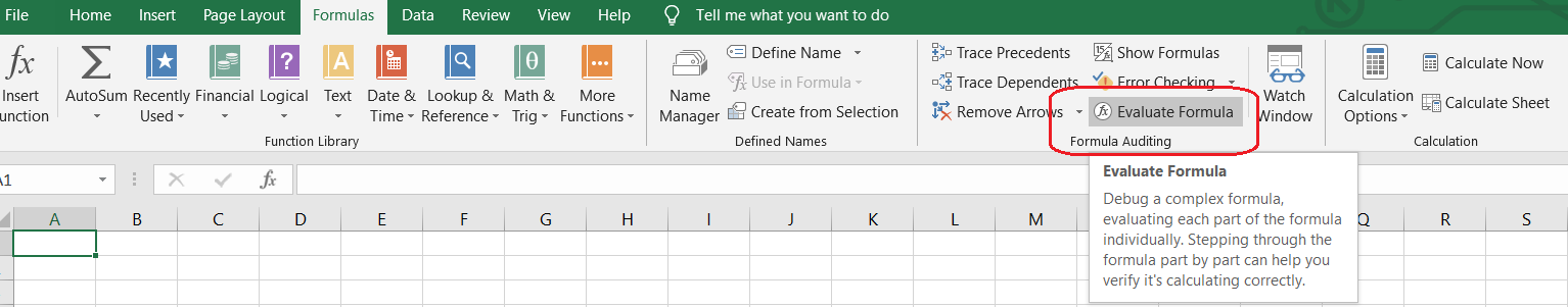
- Click the Formulas tab
- Under Formula Auditing, click Evaluate Formula
Use the Evaluate Button
Select any value from the column and click on the Evaluate Formula tool. If cell E3, for example, is selected, this dialog box pops up:
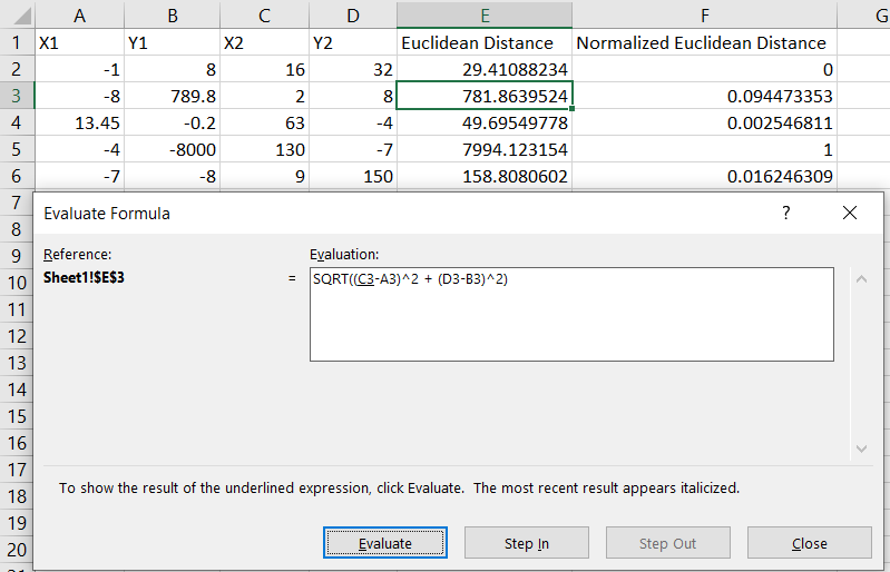
In the dialog box, you can observe the following:
- A formula (=SQRT((C3-A3)^2 + (D3-B3)^2)), which has been used to calculate the value of cell E3.
- An underline below the term C3 in the formula. This is the first term that will be evaluated in this formula. As we go further evaluating the formula, whichever term has the underline below it will be evaluated according to the given value.
- Four buttons: Evaluate, Step In, Step Out, and Close.
The Evaluate button is used to evaluate the current term according to the given value—and the value can be a formula, too.
The Step In button is nested under the current underlined term and shows what is stored inside. If the term has a formula, you can step in further until you reach a constant value.
The Step Out button is used to undo what is done by the Step In button, i.e., to move up the formula hierarchy.
You will learn how to use the Step In and Step Out buttons in the next section. In this section, focus on how the Evaluate button works. Since you have selected cell E3, which has (-8, 2) as the (X1, X2) coordinates, it will take you a total of five Evaluate button clicks to calculate the first term of the Euclidean distance. Here's the breakdown of those five steps:
- C3 evaluated to 2
- A3 evaluated to -8
- Calculating 2 - -8 which gives you 10
- Removing the round brackets around 10
- Squaring the value to arrive at 100
Similarly, go ahead and evaluate the entire formula. After a total of 12 small operations, you will arrive at the value of cell E3: 781.8639524.
Use the Step In and Step Out Buttons
In the section above, you learned how useful the Evaluate button is. In this section, you will learn how to properly use the other two buttons.
Click on any one cell (say, cell F3) from the Normalized Euclidean Distance column to open up the Evaluate dialog box. Now, before you start evaluating, notice that the underline is below the E3 term, which already has a formula in it. Therefore, click on the Step In button to reveal the underlying formula, as shown:
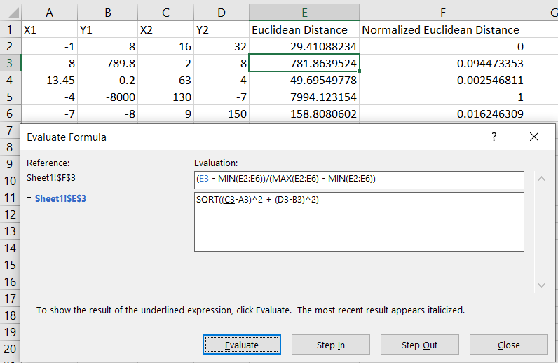
You can keep going under the formula by clicking on the Step In button until it has reach a constant value (not a formula). Since you have already evaluated the formula in cell E3 in the previous section, you know there's only one more next step to go until it reaches a constant value and thus disables the Step In button, as shown:
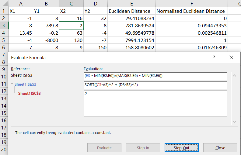
To go back to the primary formula and click on the Step Out button two times. You will now have the evaluated value of the term E3. For the next three terms, the Step In button will not be enabled because all those terms are formulas written directly in the cell F3. Evaluate the complete formula to arrive at the final result of 0.094473353 .
Conclusion
You have learned how to use the Evaluate Formula tool, including its role in breaking down a nested formula and evaluating each term step-by-step. This will help you to analyze large nested formulas and understand how they work.
Advance your tech skills today
Access courses on AI, cloud, data, security, and more—all led by industry experts.
