A Lap Around the PyData Stack
Python has become a popular alternative to R because of its clean syntax and small footprint. Let's take a look at the commonly used parts of the PyData Stack.
Sep 3, 2020 • 18 Minute Read
A Lap Around the PyData Stack
The data analytics and science community has long been dominated by the R programming language. While quite capable, R targets a niche audience. It begins to lose its appeal in the broader field of software development. In other words, no data project is an island. The modern web has made it almost mandatory that data be accessible anywhere, at any time and by anyone. The solution is to implement data solutions using a more general-purpose language.
Python has become a popular alternative to R for implementing data solutions. Python has a very small footprint with a simple, clean syntax that is easy to use and remember. Python has a very active open-source community that is contributing packages for a wide variety of tasks, including data science and analytics. And finally, Python is cross-platform. It works equally well on the three major platforms: macOS, Linux, and even Windows.
This guide is not for Python novices. It already assumes basic Python experience. However, it should be noted that someone with significant experience in another language (i.e., Java, C#) should be able to pick up Python quickly. The concepts are largely the same. Syntax is the only major difference.
The term ‘PyData’ is not official but rather a colloquial title that refers to a collection of commonly used Python packages and tools within the data science community. So while it means different things to different Pythonistas, there are a few generally accepted members of this collection. This guide will specifically focus on those and then mention several others at the end.
numpy
The numpy package handles numerical computing tasks using the Python language. Now, don't let the phrase numerical computing frighten you. You'll soon see how numpy handles most of the hard work for you. That hard work consists largely of manipulating multidimensional data structures.
Consider the task of matrix multiplication. Multiplying a 2x3 matrix with a 3x4 matrix will, after 24 multiplication operations and 8 addition operations, yield a 2x4 matrix. And this is easily done with a few lines of Python. But recall that Python is an interpreted language and can be quite slow. While it will be tough to observe a performance hit from the above example, higher dimensional data structures will quickly overwhelm pure Python.
This is why numpy is largely implemented in C. The C code compiles to native, platform specific binaries that run close to the metal, eliminating the performance issues with pure Python. But numpy still provides Python bindings to the API implemented in C. This gives the developer the best of both worlds: the performance of C and the ease of use of Python.
The central data structure of numpy is the ndarray. The “nd” stands for “n-dimensional”, so the ndarray is capable of representing multidimensional data structures. Creating an ndarray from a Python list is simple:
      import numpy as np
data = list(range(20))
arr = np.array(data)
The np alias for numpy is a common convention. You'll see it used in a lot of PyData applications. Displaying the value of arr will yield:
array([ 0, 1, 2, 3, 4, 5, 6, 7, 8, 9, 10, 11, 12, 13, 14, 15, 16, 17, 18, 19])
This looks a lot like a Python list. And the ndarray can be used as a substitute for a list much of the time. But it has learned a few new tricks. For example, the reshape method:
mat = arr.reshape(5, 4)
This will return an ndarray with the dimensions passed to it, in this case 5 rows and 4 columns:
      array([[ 0,  1,  2,  3],
       [ 4,  5,  6,  7],
       [ 8,  9, 10, 11],
       [12, 13, 14, 15],
       [16, 17, 18, 19]])
While this looks like a nested list in Python, it's actually an ndarray. Indexing an ndarray has also learned some new tricks. For example, to access the value in row 1 and column 2, you would write this code with Python lists:
mat[1][2]
This works with an ndarray as well, but there is a shortcut that reduces some of the syntactic noise.
mat[1, 2]
The cool thing about ndarray indexing is that you can select every value in a dimension with a colon, like so:
mat[:,2]
This effectively selects column two in mat. The colon says to select every row, and then index two in each row.
Another benefit of numpy is the idea of broadcasting. Consider the obligatory example of squaring a list of integers:
      my_list = list(range(10))

squares = []
for value in my_list:
  sqaure_value = value ** 2
  squares.append(square_value)
# or
squares = [value ** 2 for value in my_list]
Even though this example can be reduced to a single line of code with the list comprehension, it requires some thought to translate the Python code to the mathematical expression it represents. Using an ndarray to do the same thing is much more readable:
      my_array = np.array(list(range(10))

square_array = my_array ** 2
And numpy scales broadcasting to high dimensions as well:
      my_array = np.random.randint(0, 10, size=(3, 2))
square_array = my_array ** 2
The random module in numpy mirrors the random module in the Python standard library with some extras to accommodate the ndarray. In the above example, randint will return a 3x2 ndarray with integer values from 0 to 9.
Operations on more than one ndarray are just as easy:
      A = np.random.randint(0, 10, size=(3, 2))
B = np.random.randint(0, 10, size=(3, 2))
mat_sum = A + B
And that matrix multiplication issue mentioned at the beginning of this section?
      A = np.random.randint(0, 10, size=(2, 3))
B = np.random.randint(0, 10, size=(3, 4))
dot_prod = A.dot(B)
Finally, the ndarray can be filtered using simple Boolean expressions:
      arr = np.array(list(range(20)))
odds = arr[arr % 2 == 1]
array([ 1, 3, 5, 7, 9, 11, 13, 15, 17, 19])
This just scratches the surface of numpy. There are many other useful features (check out indexing an ndarray) that this guide cannot cover.
pandas
Hopefully you can see how powerful numpy is and how much time it can save. But at the end of the day, the ndarray is nothing more than a big glob of numbers. This is because there is no metadata associated with an ndarray. To work with data in a more intellectually palatable context, we turn to pandas.
The pandas API is what you are more likely to spend time with. While numpy handles the core operations on numeric values, pandas mimics large parts of R. This again gives you the best of both worlds: the power of R with the syntax of Python.
The central data structure in pandas is the DataFrame. It mimics the R data structure of the same name. In pandas, aDataFrame is a two-dimensional data structure with named columns and indexed rows. In other words, you can conceptually think of it as a table. The values of a DataFrame are represented by an ndarray, and a DataFrame can be created from an ndarray.
      import numpy as np
import pandas pd

raw = np.random.randint(0, 10, size=(5, 3))
df = pd.DataFrame(data=raw)
The result is
      0  1  2
0  3  4  0
1  1  8  6
2  0  5  4
3  8  5  8
4  0  1  2
The top row of headers and the left most column of indexes were generated by pandas. The headers can be modified by setting the columns field:
df.columns = ['Foo', 'Bar', 'Baz']
The DataFrame now:
      Foo  Bar  Baz
0    3    4    0
1    1    8    6
2    0    5    4
3    8    5    8
4    0    1    2
The columns can also be accessed by name:
df['Foo']
      0 3
1 1
2 0
3 8
4 0
Name: Red, dtype: int64
While bearing a strong resemblance to a DataFrame, this is actually a Series. A Series is an ndarray with an index. The column names of the DataFrame can be used as fields as well:
df.Foo
Like the ndarray a DataFrame can also be filtered.
df[df.Foo == 0]
      Foo Bar Baz
2   0   5   4
4   0   1   2
Notice that a DataFrame is returned containing the rows in which the value of Foo is zero.
A DataFrame supports dynamically adding a new column:
df['New'] = np.random.randint(0, 10, size=5)
      Foo  Bar  Baz  New
0    3    4    0    0
1    1    8    6    9
2    0    5    4    4
3    8    5    8    6
4    0    1    2    2
The DataFrame exposes a number of statistical methods such as sum:
df.sum()
      Foo    12
Bar    23
Baz    20
New    21
dtype: int64
The result is a Series with the values of the sums of the columns, and the index is the column names. To sum along the rows, add the axis= keyword argument with a value of 1 (the default is 0).
df['Total'] = df.sum(axis=1)
      Foo  Bar  Baz  New  Total
0    3    4    0    0      7
1    1    8    6    9     24
2    0    5    4    4     13
3    8    5    8    6     27
4    0    1    2    2      5
You can also change the index:
df.index = [5, 10, 15, 20, 25]
      Foo  Bar  Baz  New  Total
5     3    4    0    0      7
10    1    8    6    9     24
15    0    5    4    4     13
20    8    5    8    6     27
25    0    1    2    2      5
Accessing the rows of the DataFrame by index can be done using loc:
df.loc[15]
      Foo       0
Bar       5
Baz       4
New       4
Total    13
Name: 15, dtype: int64
And by zero-based position with iloc:
df.iloc[2]
Again, this is just scratching the surface of the capabilities of pandas.
matplotlib
It is obviously easier to use pandas over the ndarray. But most of the time, DataFrames will be very large. Presenting a DataFrame to a knowledge worker or decision maker who needs information at a glance is not an option. For this, we turn to the visualization, which is a graphical representation of data and information. Think of it as another level of abstraction.
In the PyData stack, the matplotlib package handles visualizations using Python. The matplotlib API is big, in fact it is huge. I can't begin to cover it in this guide. In fact, I have a two-hour course on Pluralsight about matplotlib that only covers an introduction to the package. But here are the basics.
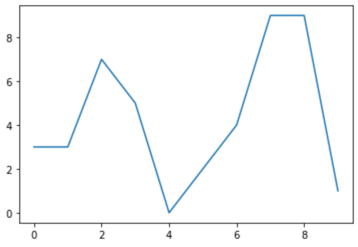
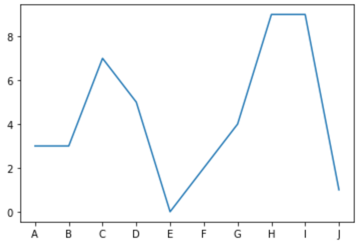
First, the module where much of the API resides is matplotlib.pyplot. This is often shortened to plt with an alias. Inside of the plt module are different functions to create different types of visualizations, such as plot to create a line chart:
      import numpy as np
import matplotlib.pyplot as plt

data = np.random.randint(0, 10, 10)
plt.plot(data)
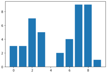
Creating a bar chart is simple as well:
plt.bar(range(len(data)), data)
Here's a pie chart:
plt.pie(data)
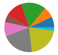
These visualizations all render the same data in different charts. With the exception of the bar chart, the functions take an ndarray or any Python iterable. For the bar function, the first argument is the positions of the bars. To space the bars evenly, just use a list of sequential integers.
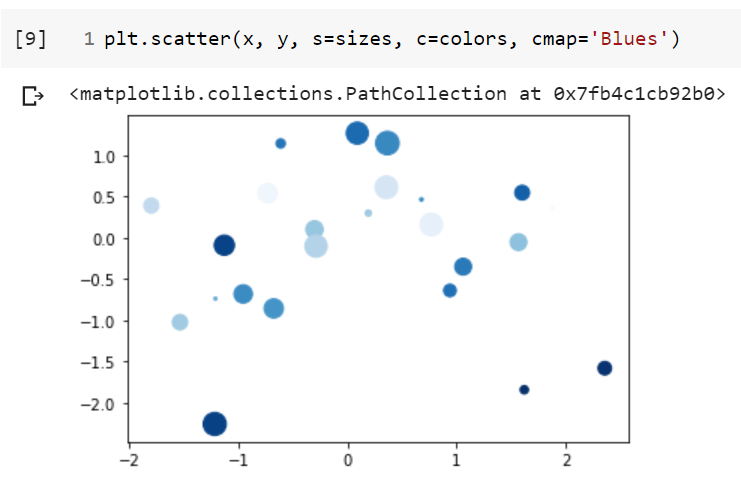
And here is a fancy scatter chart.
      x = np.random.randn(25)
y = np.random.randn(25)
colors = np.random.uniform(size=25)
sizes = np.random.uniform(size=25) * 1000
plt.scatter(x, y, c=colors, s=sizes, cmap='Blues')
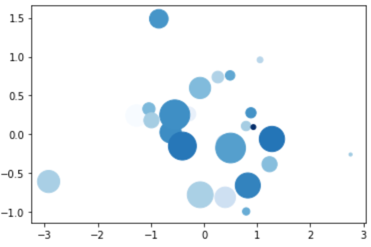
The scatter chart plots point in two dimensions. The keyword arguments c= and s= represent the color and size of the points to show the intensity of the values. The cmap= keyword argument represents the available colors to use. There are many color maps predefined in matplotlib.
You could change the values of the axes in the charts:
      import string
plt.plot(data)
labels = list(string.ascii_uppercase[:len(data)])
plt.xticks(list(range(len(labels))), labels)
Similar to the bar function, the xticks function expects the first argument to be the locations of the ticks and the second to be the new labels.
The are a number of keyword arguments in matplotlib to get the appearance of visualizations just the way you want them. You already saw some of these for the scatter chart. The line chart also provides the following:
- Color - c=
- Line Style = ls=
plt.plot(data, c='red', ls='--')
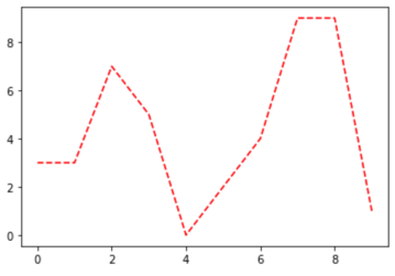
The documentation covers the complete set of keyword arguments for each visualization. As you might have guessed, there are too many to cover here.
Jupyter Notebook
The next one is a little different. It doesn't expose an API, but instead is a tool. The process of writing code in data science is not like that of most software development. In data science, you set up an experiment, set some initial parameters, run the experiment, collect the results, tweak the parameters, and repeat. This process thrives when you can get rapid feedback, and it also requires different tools.
Jupyter Notebook takes the concept of the Python REPL and goes wild with it. Instead of a platform-specific command line interface, Jupyter Notebook is like a Python session running on a web server. And you use a web browser to access that Python session. This has several advantages. You don't have to be running a specific operating system or even device to access Jupyter Notebook. You don't even need Python installed!
Also, since everything is accessed in a web browser, the results are not limited to text. The web technologies of HTML, CSS, and even JavaScript could be used to implement rich user experiences, such as:
- Syntax highlighting and automatic indentation

- Inline images with matplotlib
- Rich text with markdown

- Inline help
Jupyter Notebook also persists everything to a file in JSON. This way you can close a notebook and reopen it in the state where you last left it. It also makes sharing experiments much easier. With the Python REPL, when you close it, all of your work is lost.
I've prepared a sample notebook illustrating the concepts discussed in the previous three sections running on a service from Google called Google Colab.
Jupyter Notebook can also be installed locally via pip, but Colab is a great way to get started. And it's not a toy either. You can actually get access for free to GPUs and run jobs for up to 12 hours.
If you'd like to know more about Jupyter Notebook, check out my video course on Pluralsight: Getting Started with Jupyter Notebook and Python.
Other Packages
There are a lot of other packages often used with the packages discussed, but maybe not as often. Here are a few:
-
Scikit-Learn (sklearn): This is a machine learning API. It implements many common use cases for machine learning, such as classification and regression. Generally, it is a great choice for someone who does not need to get into the details of machine learning. You can read a Pluralsight Guide I authored about Scikit-learn for more information about it.
-
Statsmodels: Where sklearn implements common tasks in machine learning, statsmodels does the same for statistics. It provides an easy-to-use API that avoids the details of implementation.
-
Sympy: Data science will often require complex mathematical expression. While these can be written using Python, it can be difficult to read them. The sympy package is a computer algebra system that makes writing mathematical expressions in Python simpler.
-
NLTK: This is a package for implementing tasks in natural language processing. It includes an API for tagging parts of speech, parsing and tokenizing text and over 50 popular corpora (bodies of text). The nltk package even has a free, online, full-length ebook that covers the package in detail.
Summary
Data science and analytics include a diverse range of topics and skills. While R has been a popular choice of data scientists for years, in the larger field of software engineering, developers want a more general-purpose language. By using Python, developers have access to a powerful, yet simple language that avoids the quirks of R. Thanks to the open-source Python community, developers can choose from a wide selection of packages for implementing solutions to data science problems.
Advance your tech skills today
Access courses on AI, cloud, data, security, and more—all led by industry experts.
