Introduction to LSTM Units in RNN
Sep 9, 2020 • 9 Minute Read
Introduction
A previous guide explained how to execute MLP and simple RNN (recurrent neural network) models executed using the Keras API. In this guide, you will build on that learning to implement a variant of the RNN model—LSTM—on the Bitcoin Historical Dataset, tracing trends for 60 days to predict the price on the 61st day.
To predict trends more precisely, the model is dependent on longer timesteps. When training the model using a backpropagation algorithm, the problem of the vanishing gradient (fading of information) occurs, and it becomes difficult for a model to store long timesteps in its memory. In this guide, you will learn about LSTM units in RNN and how they address this problem.
Before implementing the code, let's get familiar with LSTM terms.
LSTMs
LSTM (short for long short-term memory) primarily solves the vanishing gradient problem in backpropagation. LSTMs use a gating mechanism that controls the memoizing process. Information in LSTMs can be stored, written, or read via gates that open and close. These gates store the memory in the analog format, implementing element-wise multiplication by sigmoid ranges between 0-1. Analog, being differentiable in nature, is suitable for backpropagation.
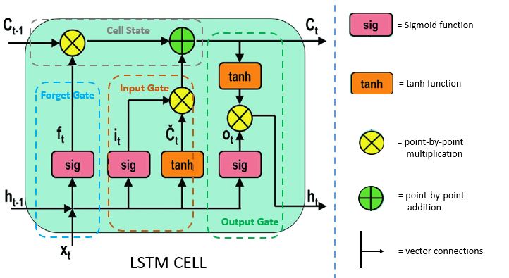
Let's look at the architecture of an LSTM.
Tanh
Tanh is a non-linear activation function. It regulates the values flowing through the network, maintaining the values between -1 and 1. To avoid information fading, a function is needed whose second derivative can survive for longer. There might be a case where some values become enormous, further causing values to be insignificant. You can see how the value 5 remains between the boundaries because of the function.
Sigmoid
Sigmoid belongs to the family of non-linear activation functions. It is contained by the gate. Unlike tanh, sigmoid maintains the values between 0 and 1. It helps the network to update or forget the data. If the multiplication results in 0, the information is considered forgotten. Similarly, the information stays if the value is 1.
This will help the network learn which data can be forgotten and which data is important to keep.
Let's learn more about these gates. There are three different gates in an LSTM cell: a forget gate, an input gate, and an output gate.
Note: All images of LSTM cells are modified from this source.
Forget Gate
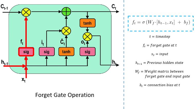
The forget gate decides which information needs attention and which can be ignored. The information from the current input X(t) and hidden state h(t-1) are passed through the sigmoid function. Sigmoid generates values between 0 and 1. It concludes whether the part of the old output is necessary (by giving the output closer to 1). This value of f(t) will later be used by the cell for point-by-point multiplication.
Input Gate
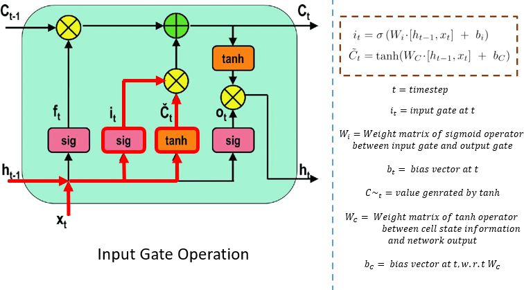
The input gate performs the following operations to update the cell status.
First, the current state X(t) and previously hidden state h(t-1) are passed into the second sigmoid function. The values are transformed between 0 (important) and 1 (not-important).
Next, the same information of the hidden state and current state will be passed through the tanh function. To regulate the network, the tanh operator will create a vector (C~(t) ) with all the possible values between -1 and 1. The output values generated form the activation functions are ready for point-by-point multiplication.
Cell State
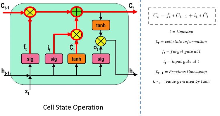
The network has enough information form the forget gate and input gate. The next step is to decide and store the information from the new state in the cell state. The previous cell state C(t-1) gets multiplied with forget vector f(t). If the outcome is 0, then values will get dropped in the cell state. Next, the network takes the output value of the input vector i(t) and performs point-by-point addition, which updates the cell state giving the network a new cell state C(t).
Output Gate
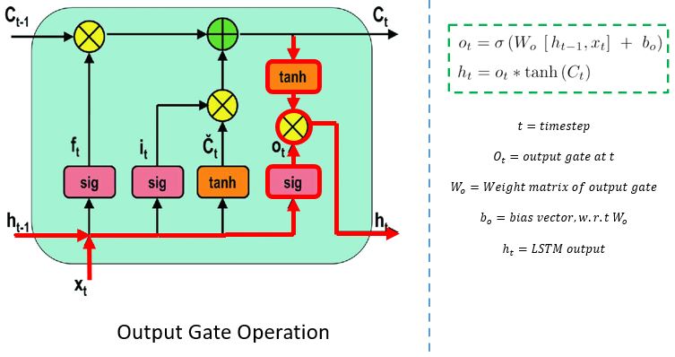
The output gate determines the value of the next hidden state. This state contains information on previous inputs.
First, the values of the current state and previous hidden state are passed into the third sigmoid function. Then the new cell state generated from the cell state is passed through the tanh function. Both these outputs are multiplied point-by-point. Based upon the final value, the network decides which information the hidden state should carry. This hidden state is used for prediction.
Finally, the new cell state and new hidden state are carried over to the next time step.
To conclude, the forget gate determines which relevant information from the prior steps is needed. The input gate decides what relevant information can be added from the current step, and the output gates finalize the next hidden state.
Let's implement the code.
Code Implementation
Note: *Refer to the code for importing important libraries and data pre-processing from this previous tutorial before building the LSTM model. *
From Keras Layers API, important classes like LSTM layer, regularization layer dropout, and core layer dense are imported.
In the first layer, where the input is of 50 units, return_sequence is kept true as it will return the sequence of vectors of dimension 50. As the return_sequence of the next layer is False, it will return the single vector of dimension 100.
from sklearn.metrics import mean_absolute_error
from keras.models import Sequential
from keras.layers import Dense, LSTM, Dropout
modell = Sequential()
modell.add(LSTM(50, return_sequences=True, input_shape=(x_train.shape[1],1)))
modell.add(Dropout(0.2))
modell.add(LSTM(100, return_sequences=False))
modell.add(Dropout(0.2))
modell.add(Dense(1))
modell.compile(loss="mean_squared_error",optimizer="rmsprop")
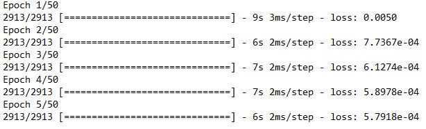
modell.fit(x_train,y_train,epochs= 50,batch_size=64)
Now test data has been prepared for prediction.
      inputs=data[len(data)-len(close_test)-timestep:]
inputs=inputs.values.reshape(-1,1)
inputs=scaler.transform(inputs)
      x_test=[]
for i in range(timestep,inputs.shape[0]):
    x_test.append(inputs[i-timestep:i,0])
x_test=np.array(x_test)
x_test=x_test.reshape(x_test.shape[0],x_test.shape[1],1)
Let's apply the model on test data.
      predicted_data=modell.predict(x_test)
predicted_data=scaler.inverse_transform(predicted_data)
      data_test=np.array(close_test)
data_test=data_test.reshape(len(data_test),1)
Time to predict.
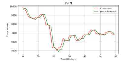
      plt.figure(figsize=(8,4), dpi=80, facecolor='w', edgecolor='k')
plt.plot(data_test,color="r",label="true-result")
plt.plot(predicted_data,color="g",label="predicted-result")
plt.legend()
plt.title("LSTM")
plt.xlabel("Time(60 days)")
plt.ylabel("Close Values")
plt.grid(True)
plt.show()
Conclusion
LSTM outperformed SimpleRNN and MLP!
The result is acceptable as the true result and predicted results are almost inline. RNNs are a good choice when it comes to processing the sequential data, but they suffer from short-term memory. Introducing the gating mechanism regulates the flow of information in RNNs and mitigates the problem.
I recommend changing the values of hyperparameters or compiling the model with different sets of optimizers such as Adam, SDG, etc., to see the change in the graph. You can also increase the layers in the LSTM network and check the results. Feel free to use this model with any other dataset.
This guide gave a brief introduction to the gating techniques involved in LSTM and implemented the model using the Keras API. Now you know how LSTM works, and the next guide will introduce gated recurrent units, or GRU, a modified version of LSTM that uses fewer parameters and output state.
Advance your tech skills today
Access courses on AI, cloud, data, security, and more—all led by industry experts.
