LSTM versus GRU Units in RNN
Sep 9, 2020 • 9 Minute Read
Introduction
Gated recurrent unit (GRU) was introduced by Cho, et al. in 2014 to solve the vanishing gradient problem faced by standard recurrent neural networks (RNN). GRU shares many properties of long short-term memory (LSTM). Both algorithms use a gating mechanism to control the memorization process.
Interestingly, GRU is less complex than LSTM and is significantly faster to compute. In this guide you will be using the Bitcoin Historical Dataset, tracing trends for 60 days to predict the price on the 61st day. If you don't already have a basic knowledge of LSTM, I would recommend reading Understanding LSTM to get a brief idea about the model.
GRU
What makes GRU special and more effective than traditional RNN?
GRU supports gating and a hidden state to control the flow of information. To solve the problem that comes up in RNN, GRU uses two gates: the update gate and the reset gate.
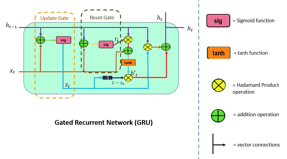
You can consider them as two vector entries (0,1) that can perform a convex combination. These combinations decide which hidden state information should be updated (passed) or reset the hidden state whenever needed. Likewise, the network learns to skip irrelevant temporary observations.
LSTM consists of three gates: the input gate, the forget gate, and the output gate. Unlike LSTM, GRU does not have an output gate and combines the input and the forget gate into a single update gate.
Let's learn more about the update and reset gates.
Update Gate
The update gate (z_t) is responsible for determining the amount of previous information (prior time steps) that needs to be passed along the next state. It is an important unit. The below schema shows the arrangement of the update gate.
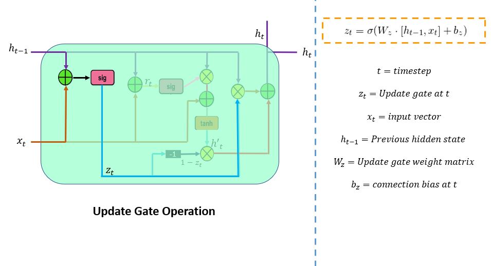
Here, x_t is the input vector served in the network unit. It is multiplied by its parameter weight (W_z) matrices. Thet_1 in h(t_1) signifies that it holds the information of the previous unit and it's multiplied by its weight. Next, the values from these parameters are added and are passed through the sigmoid activation function. Here, the sigmoid function would generate values between 0 and 1 limit.
Reset Gate
the reset gate (r_t) is used from the model to decide how much of the past information is needed to neglect. The formula is the same as the update gate. There is a difference in their weights and gate usage, which is discussed in the following section. The below schema represents the reset gate.
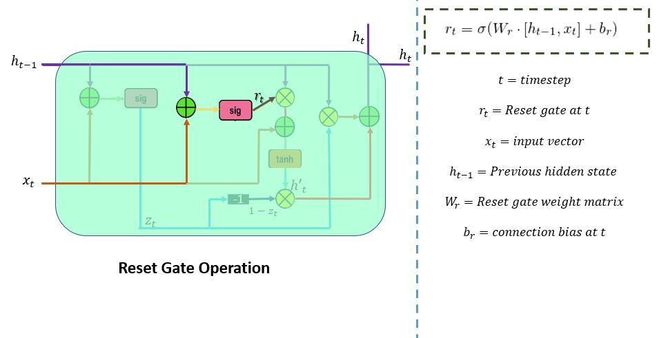
There are two inputs,x_t and h_t-1. Multiply by their weights, apply point-by-point addition, and pass it through sigmoid function.
Gates in Action
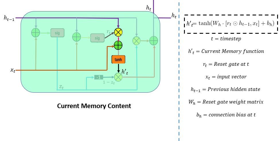
First, the reset gate stores the relevant information from the past time step into the new memory content. Then it multiplies the input vector and hidden state with their weights. Second, it calculates element-wise multiplication (Hadamard) between the reset gate and previously hidden state multiple. After summing up, the above steps non-linear activation function is applied to results, and it produces h'_t.
Consider a scenario in which a customer reviews a resort: "It was late at night when I reached here." After a couple of lines, the review ends with, "I enjoyed the stay as the room was comfortable. The staff was friendly." To determine the customer's satisfaction level, you will need the last two lines of the reviews. The model will scan the whole review to the end and assign a reset gate vector value close to '0'.
That means it will neglect the past lines and focus only on the last sentences.
Refer to the illustration below.
This is the last step. In the final memory at the current time step, the network needs to calculate h_t. Here, the update gate will play a vital role. This vector value will hold information for the current unit and pass it down to the network. It will determine which information to collect from current memory content (h't) and previous timesteps h(t-1). Element-wise multiplication (Hadamard) is applied to the update gate and h(t-1), and summing it with the Hadamard product operation between (1-z_t) and h'(t).
Revisiting the example of the resort review: This time the relevant information for prediction is mentioned at the beginning of the text. The model would set the update gate vector value close to 1. At the current time step, 1-z_t will be close to 0, and it will ignore the chunk of the last part of the review. Refer to the image below.
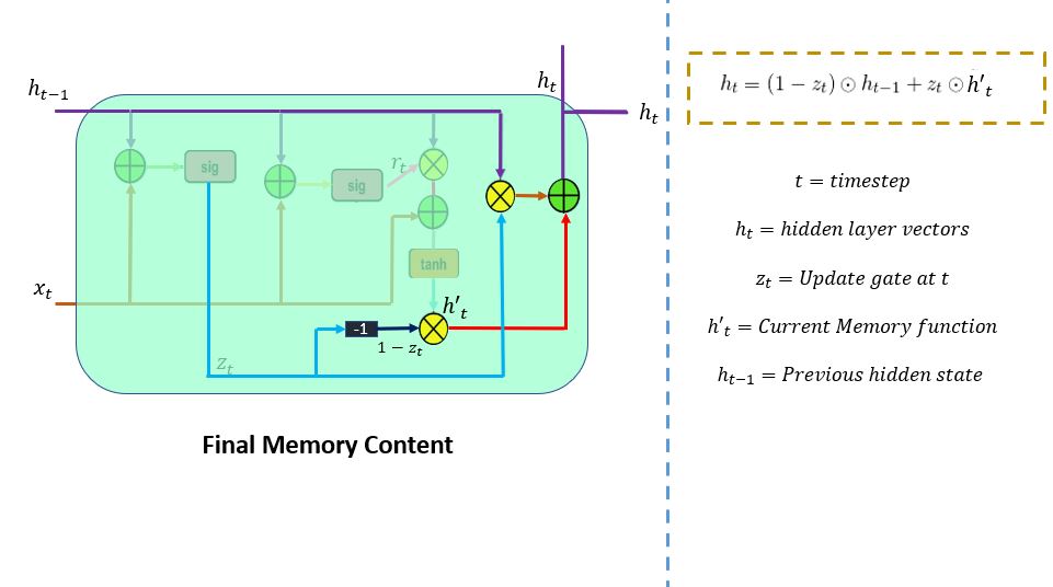
Following through, you can see z_t is used to calculate 1-z_t which, combined with h't to produce results. Hadamard product operation is carried out between h(t-1) and z_t. The output of the product is given as the input to the point-wise addition with h't to produce the final results in the hidden state.
Code Implementation
Note: Refer the code for importing important libraries and data pre-processing from this guide before building the GRU model.
From Keras Layers API, import the GRU layer class, regularization layer: dropout and core layer dense.
In the first layer where the input is of 50 units, return_sequence is kept true as it returns the sequence of vectors of dimension 50. The return_sequence of the next layer would give the single vector of dimension 100.
from sklearn.metrics import mean_absolute_error
from keras.models import Sequential
from keras.layers import Dense, GRU, Dropout
mode = Sequential()
mode.add(GRU(50, return_sequences=True, input_shape=(x_train.shape[1],1)))
mode.add(Dropout(0.2))
mode.add(GRU(100,return_sequences=False))
mode.add(Dropout(0.2))
mode.add(Dense(1, activation = "linear"))
mode.compile(loss="mean_squared_error",optimizer="rmsprop")
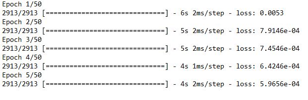
mode.fit(x_train,y_train,epochs= 50,batch_size=64)
Now test data has prepared for prediction.
      inputs=data[len(data)-len(close_test)-timestep:]
inputs=inputs.values.reshape(-1,1)
inputs=scaler.transform(inputs)
      x_test=[]
for i in range(timestep,inputs.shape[0]):
    x_test.append(inputs[i-timestep:i,0])
x_test=np.array(x_test)
x_test=x_test.reshape(x_test.shape[0],x_test.shape[1],1)
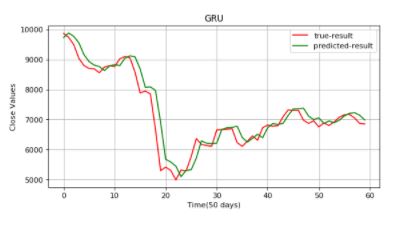
Let's apply the model on test data. Time to predict.
      plt.figure(figsize=(8,4), dpi=80, facecolor='w', edgecolor='k')
plt.plot(data_test,color="r",label="true-result")
plt.plot(predicted_data,color="g",label="predicted-result")
plt.legend()
plt.title("GRU")
plt.xlabel("Time(60 days)")
plt.ylabel("Close Values")
plt.grid(True)
plt.show()
      predicted_data=mode.predict(x_test)
predicted_data=scaler.inverse_transform(predicted_data)
      data_test=np.array(close_test)
data_test=data_test.reshape(len(data_test),1)
      plt.figure(figsize=(8,4), dpi=80, facecolor='w', edgecolor='k')
plt.plot(data_test,color="r",label="true-result")
plt.plot(predicted_data,color="g",label="predicted-result")
plt.legend()
plt.title("GRU")
plt.xlabel("Time(60 days)")
plt.ylabel("Close Values")
plt.grid(True)
plt.show()
Conclusion
To sum up, GRU outperformed traditional RNN. If you compare the results with LSTM, GRU has used fewer tensor operations. It takes less time to train. The results of the two, however, are almost the same. There isn't a clear answer which variant performed better. Usually, you can try both algorithms and conclude which one works better.
This guide was a brief walkthrough of GRU and the gating mechanism it uses to filter and store information. A model doesn't fade information—it keeps the relevant information and passes it down to the next time step, so it avoids the problem of vanishing gradients. LSTM and GRU are state-of-the-art models. If trained carefully, they perform exceptionally well in complex scenarios like speech recognition and synthesis, neural language processing, and deep learning.
For further study, I recommend reading this paper, which clearly explains the distinction between GRU and LSTM.
Advance your tech skills today
Access courses on AI, cloud, data, security, and more—all led by industry experts.
