Expediting Deep Learning with Transfer Learning: PyTorch Playbook
Jul 16, 2020 • 11 Minute Read
Introduction
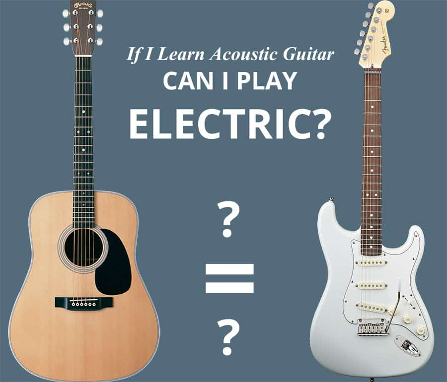
Yes! It is easier for you to learn how to play the electronic guitar if you already know how to play the acoustic guitar. You don't have to learn the basics of electric guitar again from the beginning. We humans can intelligently apply knowledge learned previously to a different task or domain and use that knowledge to solve new problems effectively.
Can a machine imitate this knowledge transferring power of the human brain? Yes, thanks to transfer learning (TL).
This guide will cover the motivation and types of TL. For a brief introduction to pre-trained models and a hands-on example, check out this Kaggel competition, Dogs vs Cats. As it is a two-class classification, in machine learning terms it is known as a binary classification problem.
Motivation
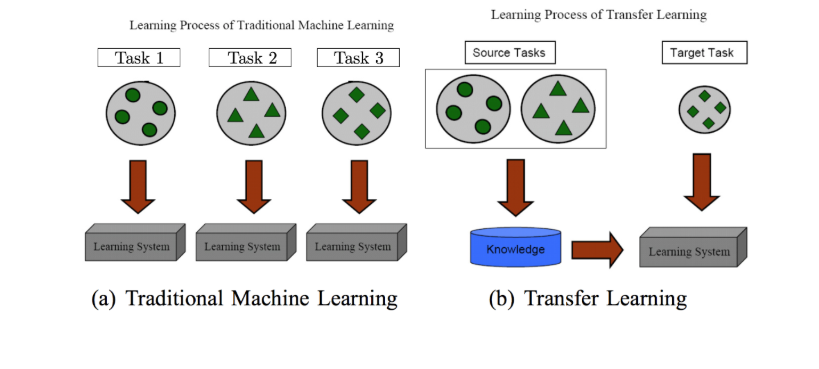
Transfer learning has an emphasis on storing the knowledge gained while solving one task and applying it to different but related tasks. A basic learning process is shown below.
Traditionally, CNN and deep learning algorithms are used for solving specific tasks. Once the feature-space distribution changes, the model needs to be built from scratch. The initial layers in the convolution network detect the low-level features like intensities, colors, edges, etc. Whether you are detecting a car, human, or animal, these layers are common. The deeper layers will detect more complex features like shape, face, pattern, etc.
The bigger the training data the better the prediction accuracy will be. While working on complex problems, humongous training image data is required. That means stacking more and more layers to make the network deeper. But suppose stacking 1000 neural network (NN) layers doesn't yield good results, and made the situation worse.
Transfer learning to the rescue!
Instead of creating the whole network from scratch, the model can learn the features of one task and apply them to another. It is common to use a pre-trained model. Most commonly these models have trained on ImageNet--1.2 million images with 1000 categories.
Remember to change your classification layer (FC) to the same number of classes that you need to predict.
Types of Transfer Learning Techniques
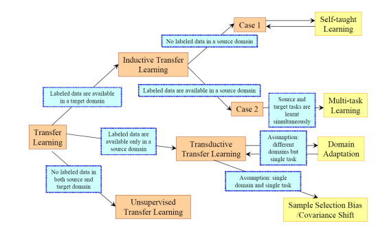
There are three types of TL techniques: Inductive, Transductive, and Unsupervised. Below is an overview of different settings to transfer.
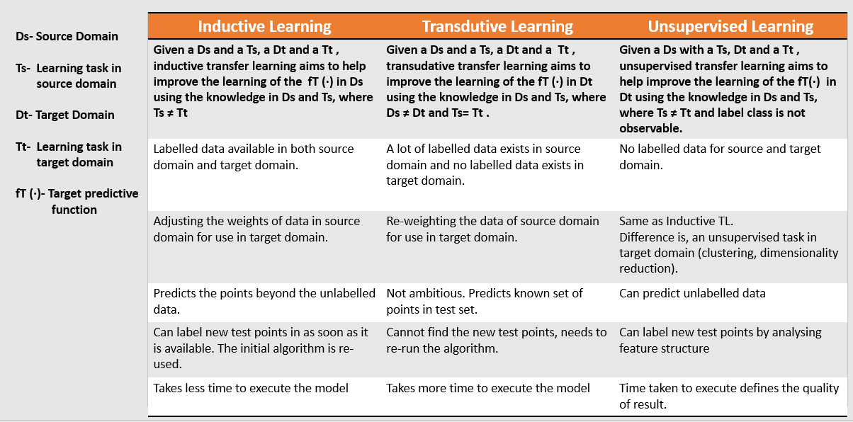
Their definitions and differences are given below.
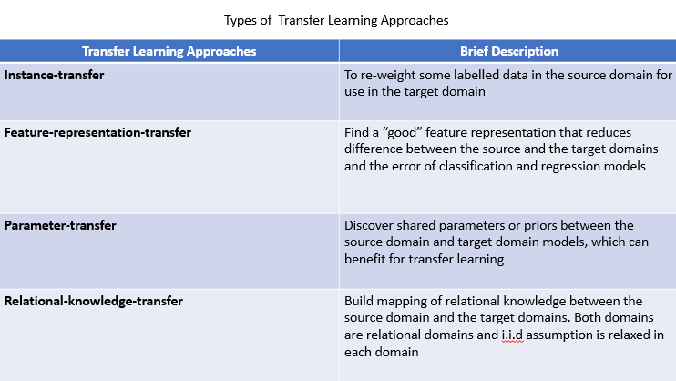
The image below shows the different approaches to implement TL from the source domain to the target domain
Applying Transfer Learning
What
Understand the common knowledge between source and target domain/task to improve the performance of the target task.
When
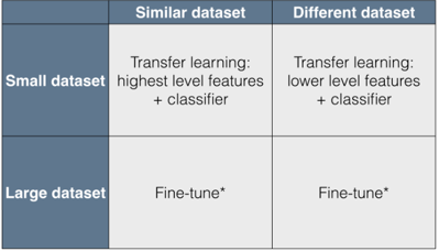
It is suggested not to use TL if your target dataset is distinct from the training dataset (ImageNet), which is generally not the case considering the variety of images. This type of knowledge transfer is known as negative transfer. ImageNet weights will not help if target images are out of their scope, for example, medical images or images from a telescope.
How
When the source and target domains and tasks are related, identify the different transfer learning techniques.
Follow the table below and match your requirements.
Now you'll learn how to apply these TL techniques to Deep Learning.
Apply Transfer Learning in Deep Learning
Pre-trained Models
Deep learning requires a good amount of training time and data compared to machine learning (computer vision). You can save some time using pre-trained models to extract the features, fine-tune their weights, save them, and make them available for others to use. This is also known as deep transfer learning
Below are some famous types of pre-trained models available to download at Pytorch API.
- ResNet
- DenseNet
- VGG-16
- MobileNet
Pre-trained models will give the benefits of high accuracy and speed, saving you from weeks of work to train and create these models from scratch.
Fine-tuning
The deeper layers of pre-trained models are used for learning features and are fine-tuned. To implement transfer learning with fine-tuning, the last layers are replaced when the trainable layer is added.
The earlier layers are more generalized even if the data is new and small. The results would come out absolutely fine even if you freeze the initial layers and retain the rest. For larger datasets, you may retain the complete network with initial weights.
This guide will use a DenseNet121 pre-trained model as a feature extractor. The data has a constraint of having fewer training samples per category. Even if the input images are new and never existed before in ImageNet, the model has to extract appropriate features and predict the results.
Implementation in Python
Import the important libraries.
      import torchvision
import torch.nn as nn
import torch
import torch.nn.functional as F
from torchvision import transforms,models,datasets
import matplotlib.pyplot as plt
from PIL import Image
import numpy as np
from torch import optim
Call the images and transform using the transform.Compose function.
      train_data_dir = '/input/cat-and-dog/training_set/training_set'

transform = transforms.Compose([transforms.Resize(255),
    transforms.CenterCrop(224),
    transforms.ToTensor()])

dataset = torchvision.datasets.ImageFolder(train_data_dir, transform= transform)
train_loader = torch.utils.data.DataLoader(dataset, batch_size=400 ,shuffle=True)
test_data_dir = '/input/cat-and-dog/test_set/test_set'

transform = transforms.Compose([transforms.Resize(255),
    transforms.CenterCrop(224),
    transforms.ToTensor()])

test_dataset = torchvision.datasets.ImageFolder(test_data_dir, transform= transform)
test_loader = torch.utils.data.DataLoader(dataset, batch_size=400 ,shuffle=True)
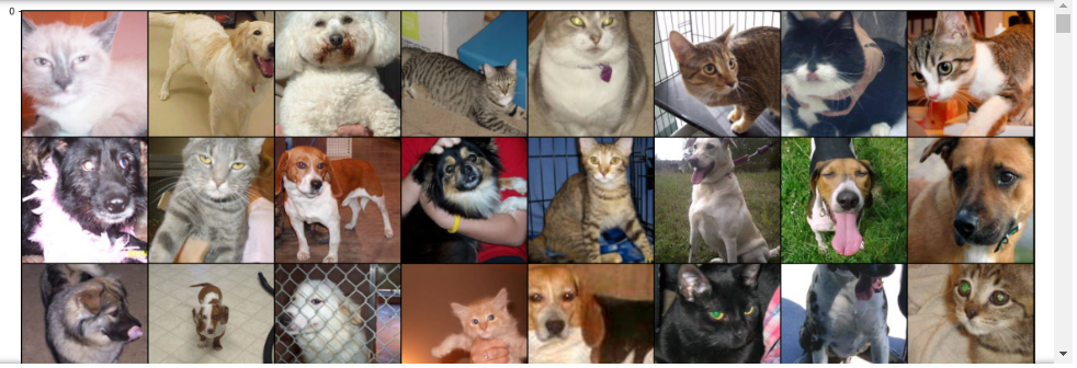
      def imshow(inp, title=None):
    """Imshow for Tensor."""
    inp = inp.numpy().transpose((1, 2, 0))
    plt.figure(figsize=(20,150))
    plt.imshow(inp)

inputs, classes = next(iter(train_loader))

# Make a grid from batch
out = torchvision.utils.make_grid(inputs, scale_each= True)

imshow(out)
Download the pre-trained model.
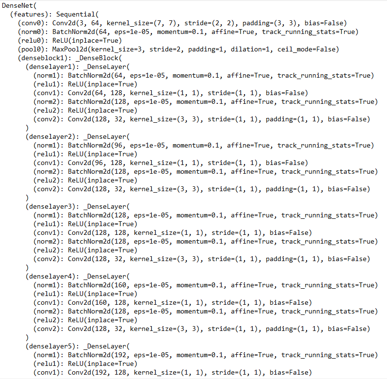
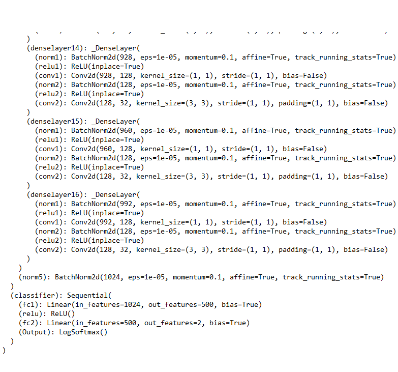
      model = models.densenet121(pretrained = True)
model
Change the output layer with an activation layer of Logsoftmax().
      for params in model.parameters():
    params.requires_grad = False

from collections import OrderedDict

classifier = nn.Sequential(OrderedDict([
    ('fc1',nn.Linear(1024,500)),
    ('relu',nn.ReLU()),
    ('fc2',nn.Linear(500,2)),
    ('Output',nn.LogSoftmax(dim=1))
]))

model.classifier = classifier
Train the model.
      model = model.cuda()
optimizer= optim.Adam(model.classifier.parameters())
criterian= nn.NLLLoss()
list_train_loss=[]
list_test_loss=[]

for epoch in range(10):
    train_loss= 0
    test_loss= 0
    for bat,(img,label) in enumerate(train_loader):
        # moving batch and labels to gpu
        img = img.to('cuda:0')
        label = label.to('cuda:0')
        model.train()
        optimizer.zero_grad()

        output = model(img)
        loss = criterian(output,label)
        loss.backward()
        optimizer.step()
        train_loss = train_loss+loss.item()

    accuracy=0
    for bat,(img,label) in enumerate(test_loader):
        img = img.to('cuda:0')
        label = label.to('cuda:0')
        model.eval()
        logps= model(img)
        loss = criterian(logps,label)
        test_loss+= loss.item()
        ps=torch.exp(logps)
        top_ps,top_class=ps.topk(1,dim=1)
        equality=top_class == label.view(*top_class.shape)
        accuracy +=torch.mean(equality.type(torch.FloatTensor)).item()

    list_train_loss.append(train_loss/20)
    list_test_loss.append(test_loss/20)
    print('epoch: ',epoch,' train_loss: ',train_loss/20,' test_loss: ',test_loss/20,' accuracy: ', accuracy/len(test_loader))
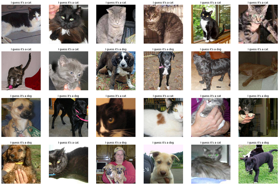
      samples, _ = iter(test_loader).next()
samples = samples.to('cuda:0')
fig = plt.figure(figsize=(24, 16))
fig.tight_layout()
output = model(samples[:24])
pred = torch.argmax(output, dim=1)
pred = [p.item() for p in pred]
ad = {0:'I guess it\'s a cat', 1:'I guess it\'s a dog'}
for num, sample in enumerate(samples[:24]):
    plt.subplot(4,6,num+1)
    plt.title(ad[pred[num]])
    plt.axis('off')
    sample = sample.cpu().numpy()
    plt.imshow(np.transpose(sample, (1,2,0)))
      import matplotlib.pyplot as plt
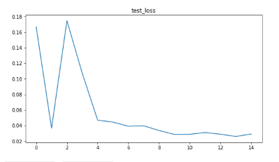
figs , ax = plt.subplots(1,2,figsize=(20,5))
ax[0].plot(list_test_loss)
ax[0].set_title('test_loss')
Well done! The accuracy is 99%.
Conclusion
The objective of this guide is to give a brief introduction to transfer learning and its types and approaches, as well as how it can be applied in deep learning. Check out the links provided in this guide for the different pre-trained models for deep learning, and try executing them on the cat and dog dataset. I encourage you to apply this model in your own dataset, but make sure you change the classification layer as per the problem statement.
I hope you learned something new today. Happy learning!
Advance your tech skills today
Access courses on AI, cloud, data, security, and more—all led by industry experts.

