Basic Time Series Algorithms and Statistical Assumptions in Python

May 15, 2020 • 11 Minute Read

Introduction

Time series algorithms are extensively used for analyzing and forecasting time-based data. These algorithms are built on underlying statistical assumptions. In this guide, you will learn the statistical assumptions and the basic time series algorithms, and their implementation in Python.

Let's begin by understanding the data.

Data

In this guide, you will use the fictitious monthly sales data of a supermarket chain containing 564 observations and three variables, as described below:

date: the first date of every month
sales: daily sales, in millions of dollars
Class: the variable denoting the training and test data set partition

The lines of code below import the required libraries and the data.

      import pandas as pd
import numpy as np 

# Reading the data
df = pd.read_csv("timeseries2.csv")
print(df.shape)
print(df.info())
    

Output:

      (564, 3)
    
    <class 'pandas.core.frame.DataFrame'>
    RangeIndex: 564 entries, 0 to 563
    Data columns (total 3 columns):
    date     564 non-null object
    sales    564 non-null float64
    Class    564 non-null object
    dtypes: float64(1), object(2)
    memory usage: 13.3+ KB
    None
    

The next step is to create the training and test datasets for model validation. You will also create the training array that will be used for statistical tests.

      train = df[df["Class"] == "Train"]
test = df[df["Class"] == "Test"]
print(train.shape)
print(test.shape)

train_array = train["sales"]
print(train_array.shape)
    

Output:

      (552, 3)
    (12, 3)

    (552,)
    

With the data prepared, you are ready to move to the forecasting techniques in the subsequent sections. However, before moving to forecasting it's important to understand the statistical concepts of white noise and stationarity in time series.

White Noise

A white noise series is a time series that is purely random and has variables that are independent and identically distributed with a mean of zero. This means that the observations have the same variance and there is no auto-correlation.

One of the initial techniques is to look at the summary statistics. This can be done with the code below. The output shows that the mean is not zero and the standard deviation is not one. These numbers indicate that the series is not white noise.

      print(train_array.describe())

Output:

      count    552.000000
    mean       6.221014
    std        2.105854
    min        2.100000
    25%        5.000000
    50%        6.000000
    75%        6.900000
    max       12.300000
    Name: sales, dtype: float64
    

Visualizing the series is the next step, and can be done using the code below.

      import matplotlib.pyplot as plt
train_array.plot()
plt.show()
    

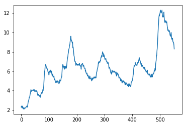
The information in this visualization shows that the data is not a purely random series. You can also create a histogram to confirm whether the distribution is normal.

      # histogram plot
train_array.hist()
plt.show()
    

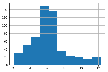
Both the above plots confirm that the series is not white noise. Another method of confirming this is through auto-correlation, which is expected to be zero. This can be visualized with the code below.

      from pandas.plotting import autocorrelation_plot
autocorrelation_plot(train_array)
plt.show()
    

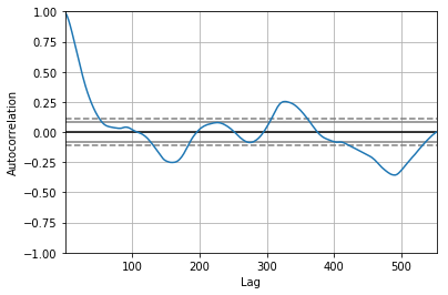
The output above shows a significant autocorrelation pattern. All of the above analysis suggests that this is not a white noise series.

Stationary Series

One of the popular time series algorithms is the Auto Regressive Integrated Moving Average (ARIMA), which is defined for stationary series. A stationary series is one where the properties do not change over time. There are several methods to check the stationarity of the series. The one you’ll use here is the Augmented Dickey-Fuller test.

Augmented Dickey-Fuller Test

The Augmented Dickey-Fuller test is a type of statistical unit root test. The test uses an autoregressive model and optimizes an information criterion across multiple different lag values.

The null hypothesis of the test is that the time series is not stationary, whereas the alternate hypothesis (rejecting the null hypothesis) is that the time series is stationary.

The first step is to import the adfuller module from the statsmodels package. This is done in the first line of code below. The second line creates a series of values using the sales variable of the training data set. The remaining lines conducts the test and prints the result values.

      from statsmodels.tsa.stattools import adfuller

X = train.sales

result = adfuller(X)
print('ADF Statistic: %f' % result[0])
print('p-value: %f' % result[1])
print('Critical Values:')
for key, value in result[4].items():
    print('\t%s: %.3f' % (key, value))
    

Output:

      ADF Statistic: -2.960313
    p-value: 0.038771
    Critical Values:
    	1%: -3.442
    	5%: -2.867
    	10%: -2.570
    

The output above shows that the p-value is slightly lower than the threshold value of 0.05 which means you reject the null hypothesis. The series seems to be roughly stationary. Having understood the basic statistical concepts of time series, you will now build time series forecasting models.

One last step before building the model is to create a utility function that will be used as an evaluation metric. The code below creates the function for calculating the mean absolute percentage error (MAPE), which is the metric to be used. The lower the MAPE value, the better the forecasting model performance.

      def mean_absolute_percentage_error(y_true, y_pred): 
    y_true, y_pred = np.array(y_true), np.array(y_pred)
    return np.mean(np.abs((y_true - y_pred) / y_true)) * 100
    

Simple Exponential Smoothing

In the exponential smoothing method, forecasts are produced using weighted averages of past observations, with the weights decaying exponentially as the observations get older. The value of the smoothing parameter for the level is decided by the parameter smoothing_level.

The first two lines of code below import the required libraries and the modules. The third line fits the simple exponential model, while the fourth line generates the forecast on the test data. Finally, the mean_absolute_percentage_error() function is used to produce the MAPE error on the test data, which comes out to be 10%.

      import statsmodels.api as sm
from statsmodels.tsa.api import ExponentialSmoothing, SimpleExpSmoothing, Holt

model1 = SimpleExpSmoothing(np.asarray(train['sales'])).fit(smoothing_level=0.7,optimized=False)

test['SimpleExp'] = model1.forecast(len(test))
mean_absolute_percentage_error(test.sales, test.SimpleExp)
    

Output:

      10.05

Holt Linear Trend

This is an extension of the simple exponential smoothing method that takes into account the trend component while generating forecasts. This method involves two smoothing equations, one for the level and one for the trend component.

The lines of code below create the model on the training data, generate predictions on the test data, and evaluate the model performance using the utility function.

      fit_holt = Holt(np.asarray(train['sales'])).fit(smoothing_level = 0.5,smoothing_slope = 0.1)

test['Holt_linear_model'] = fit_holt.forecast(len(test))

mean_absolute_percentage_error(test.sales, test.Holt_linear_model)

Output:

      2.15

The output above shows that the MAPE for the test data is 2.1%.

Holt-Winters Method

This is an extension of the holt-linear model that takes into account both the trend and seasonality component while generating forecasts.

The lines of code below create the model on the training data, generate predictions on the test data, and evaluate the model performance using the utility function.

      fit_holt_winter = ExponentialSmoothing(np.asarray(train['sales']) ,seasonal_periods=6 ,trend='add', seasonal='add',).fit()

test['Holt_Winter'] = fit_holt_winter.forecast(len(test))

mean_absolute_percentage_error(test.sales, test.Holt_Winter)

Output:

      6.837

The output above shows that the MAPE for the test data is 6.8%.

Conclusion

In this guide, you learned about the underlying statistical concepts of white noise and stationarity in time series data. You also learned how to implement basic time series forecasting models using Python.

The performance of the models on the test data is summarized below:

Simple Exponential Smoothing: MAPE of 10%
Holt Linear Trend Model: MAPE of 2.1%
Holt-Winters Method: MAPE of 6.8%

The simple exponential smoothing model did well to achieve a lower MAPE of 10%. However, the other two models outperformed it by producing an even lower MAPE. The Holt Linear Trend model emerged as the winner based on its lowest MAPE of 2.1%.

To learn more about data science using Python, please refer to the following guides.