Getting Started with Azure ML Studio
Jun 5, 2020 • 12 Minute Read
Introduction
Azure Machine Learning Studio (ML Studio) is a graphical, collaborative, drag-and-drop web interface from Microsoft for building machine learning models. It does not require coding knowledge of R or Python, and the cloud interface can be used to build models through ML Studio.
ML Studio contains all the necessary features required to design, develop, train, evaluate, and share the machine learning model. In this guide, you will learn about the basics of Azure ML Studio. It comes with a free subscription and provides sufficient free space to follow through the topics covered in this guide. In order to create a free subscription, you can visit this link.
The following sections will guide you through six steps to build a machine learning model with Azure ML Studio.
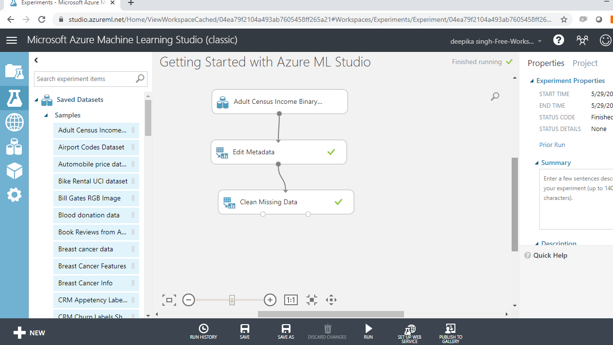
Step One: Load Data
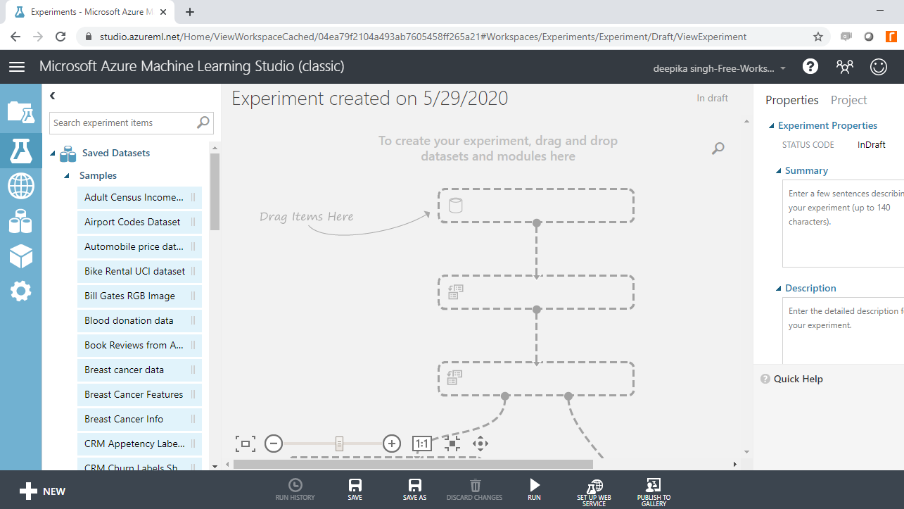
After completing the subscription procedure and opening ML Studio, you will see the following window.
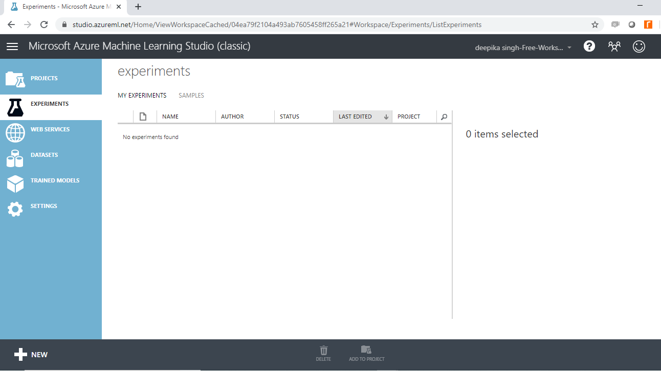
In the above image, there are many features listed on the left sidebar. You’ll use the Experiments feature for building the machine learning model.
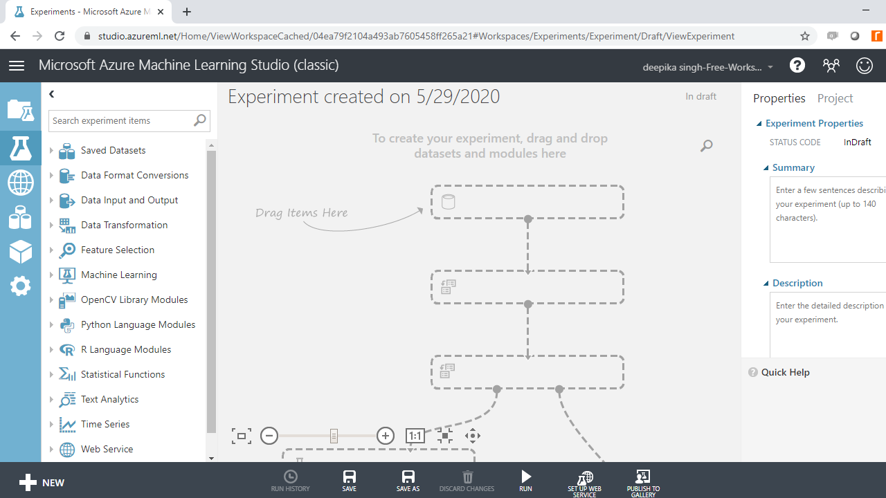
To start, click on the Experiments option, followed by the New button. Next, click on the blank experiment and the following screen will be displayed.
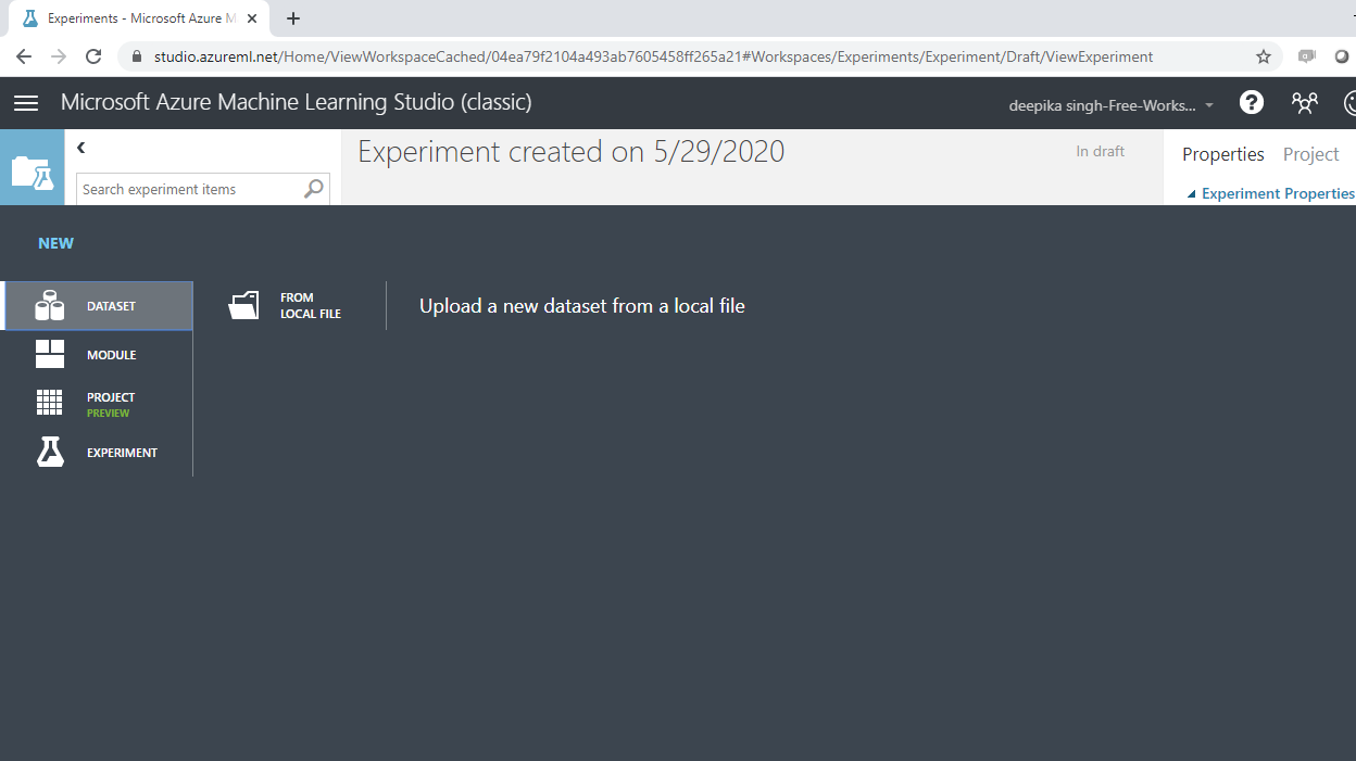
You are ready to load the data. There are many options available for data import. For example, if you want to upload the file from the local system, click New, and select the Dataset option, as shown below.
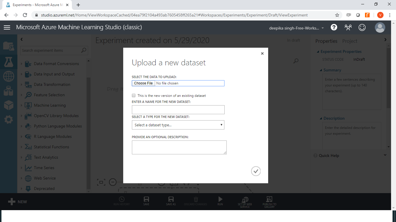
The above selection will open the window shown below, which can be used to upload the dataset from the local system.
You can also use the in-built dataset provided in ML Studio. To do this, click on the Saved Datasets option from the workspace as shown below.
This will open the list of datasets available in ML Studio.
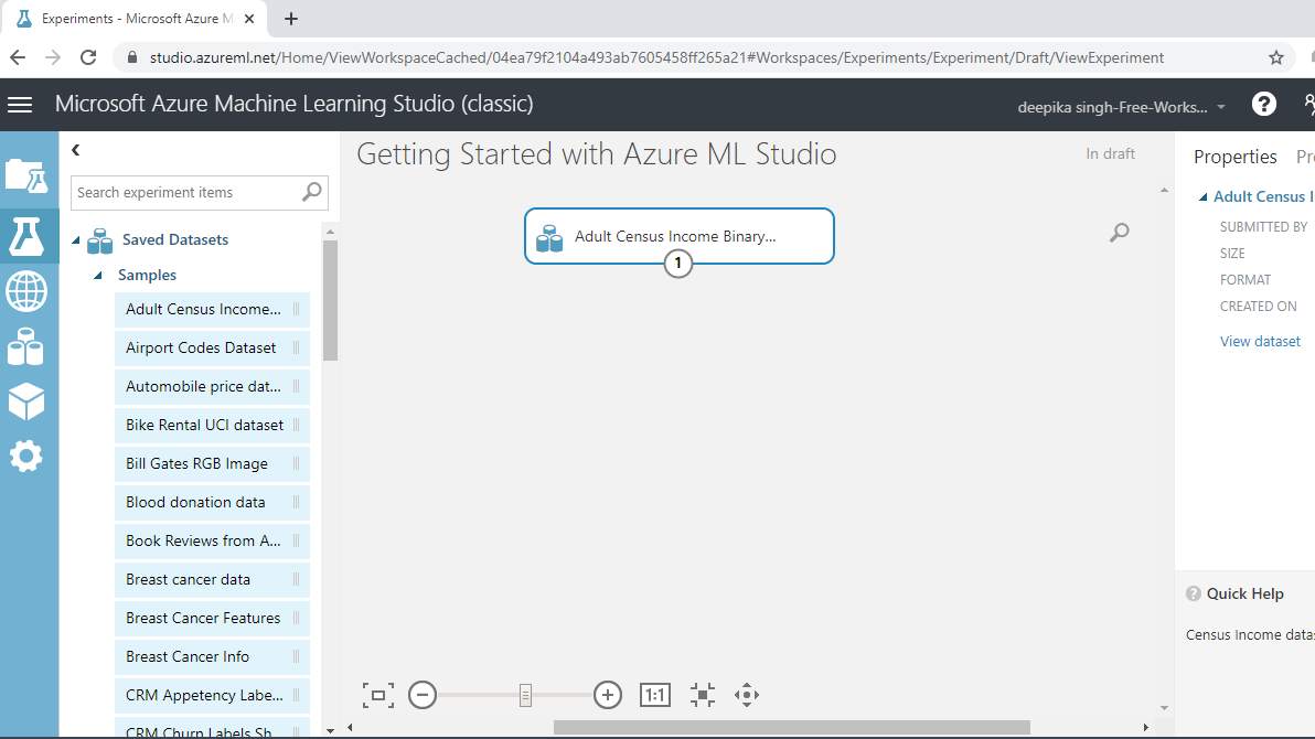
Drag the Adult Census Income Binary Classification dataset from the Saved Datasets list into the workspace and name it "Getting Started with Azure ML Studio".
Understanding the Data
The Adult Census Income Binary Classification dataset is a subset of the 1994 census database, using working adults over the age of 16 with an adjusted income index of greater than 100. The data is used as a classification machine learning problem where the objective is to classify people using demographics to predict whether a person earns over US$50,000 a year. The data comes from UCI Machine Learning Repository.
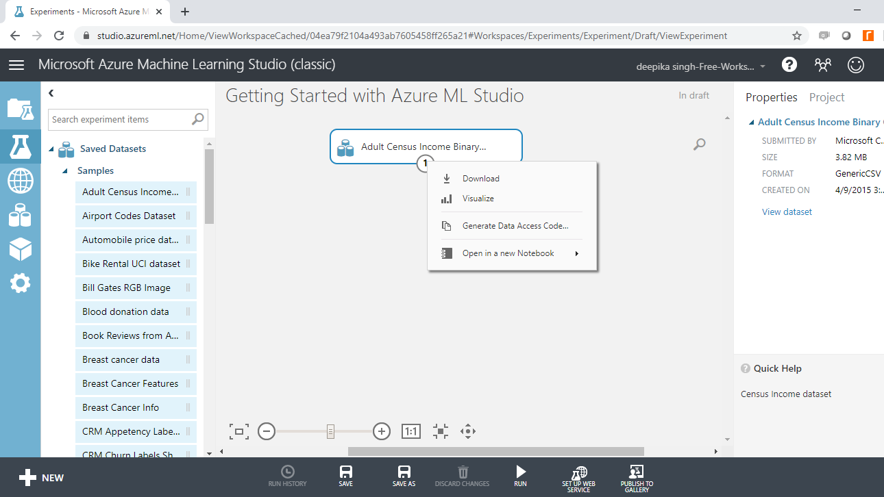
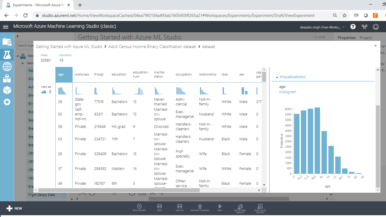
To understand more about the data, you can right click and select the Visualize option as shown below.
The above selection opens the window shown below. There are 32561 rows and 15 columns. Selecting any variable will display its Statistics as shown below.
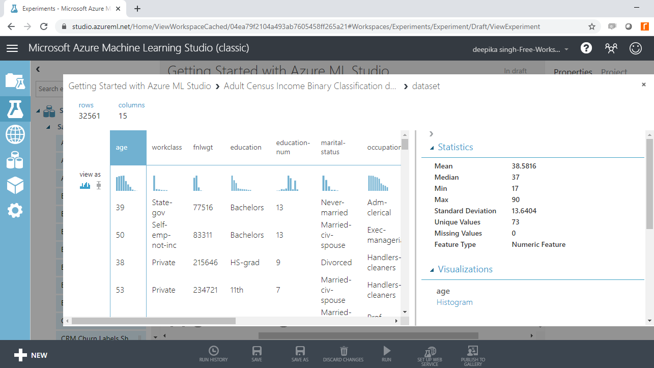
Scrolling down will display the Visualizations of the selected variable. In this case, the histogram of age is displayed.
Step Two: Prepare Data for Modeling
Before building the classification model, data preparation is required. To start, convert the string variables to categorical. Start by typing "edit metadata" in the search bar to find the Edit Metadata module, and then drag it into the workspace.
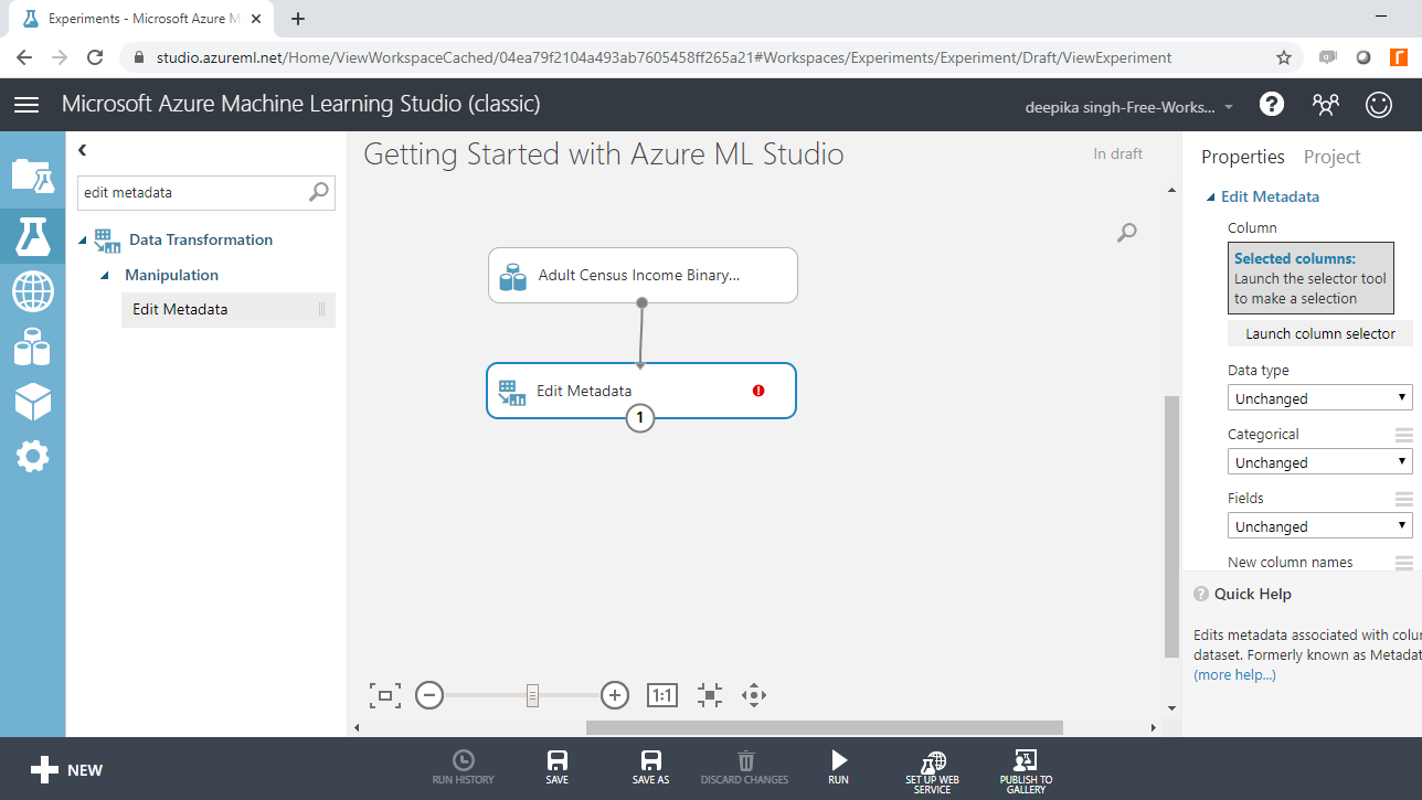
The next step is to click on the Launch column selector option placed in the righthand side of the workspace and select the string variables from the available columns. This will generate the output below.
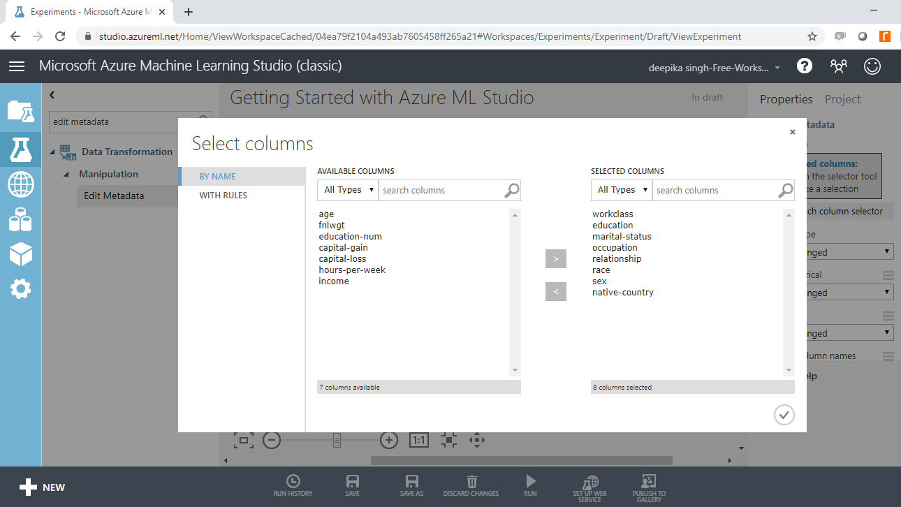
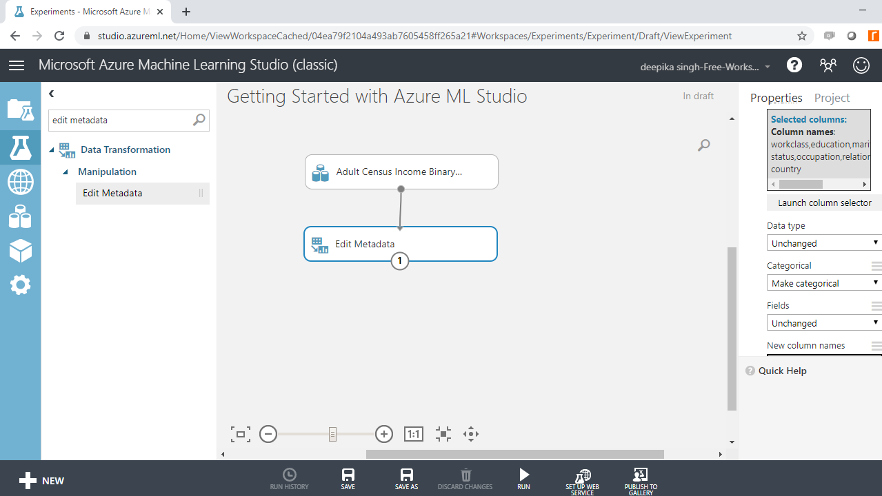
Once you have made selections, the selected columns will be displayed in the workspace. Next, from the dropdown options under Categorical, select the Make categorical option. Next, click on the Run button at the bottom of the workspace, which is used in ML Studio to execute the modules in the workspace. If there is no error in any module, the experiment run is completed and you will see a green tick mark.
Missing Value Treatment
One of the common data preparation tasks is to treat missing values. Start by searching and dragging the Clean Missing Data module into the experiment workspace.
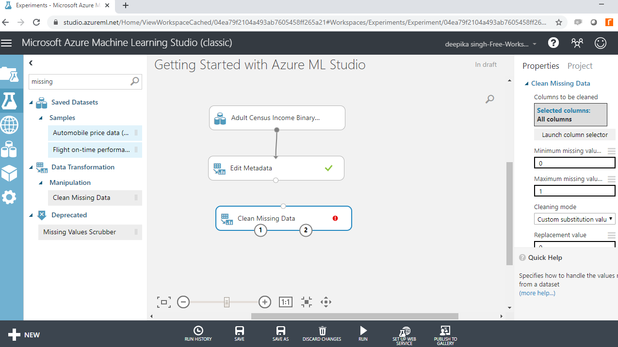
Next, connect the output port of the Edit Metadata module with the input port of the Clean Missing Data module.
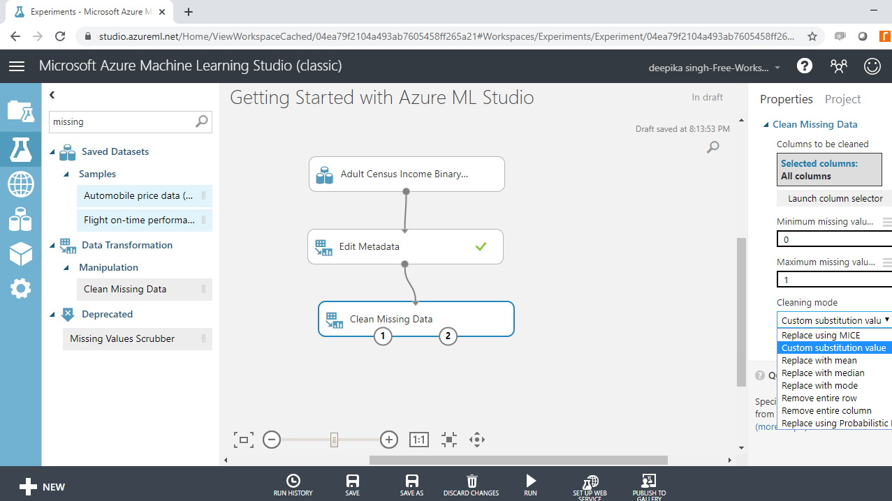
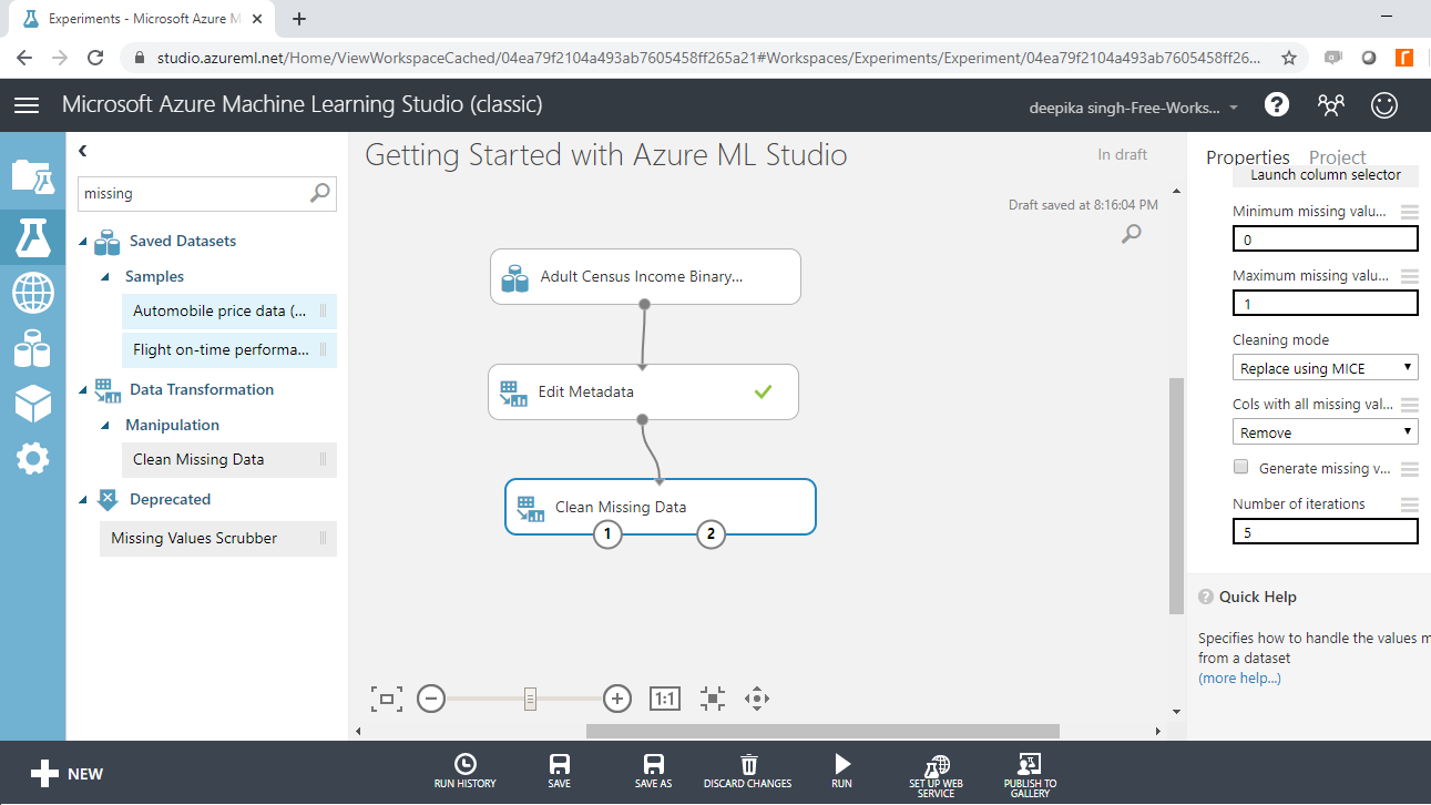
On the right hand side of the workspace, there are different options for performing the Clean Missing Data operation. There are several methods of dealing with missing values. One of the advanced techniques is using the MICE technique. MICE stands for Multivariate Imputation by Chained Equations and it works by creating multiple imputations (replacement values) for multivariate missing data. Under the Cleaning mode tab, select the Replace using MICE option as shown below. Keep all the other options as default.
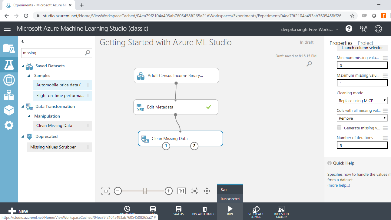
Next, click on the Run tab, and select the Run selected option. This will only run the module that is still not executed.
The missing data operation is performed, as is evident from the green tick in the module.
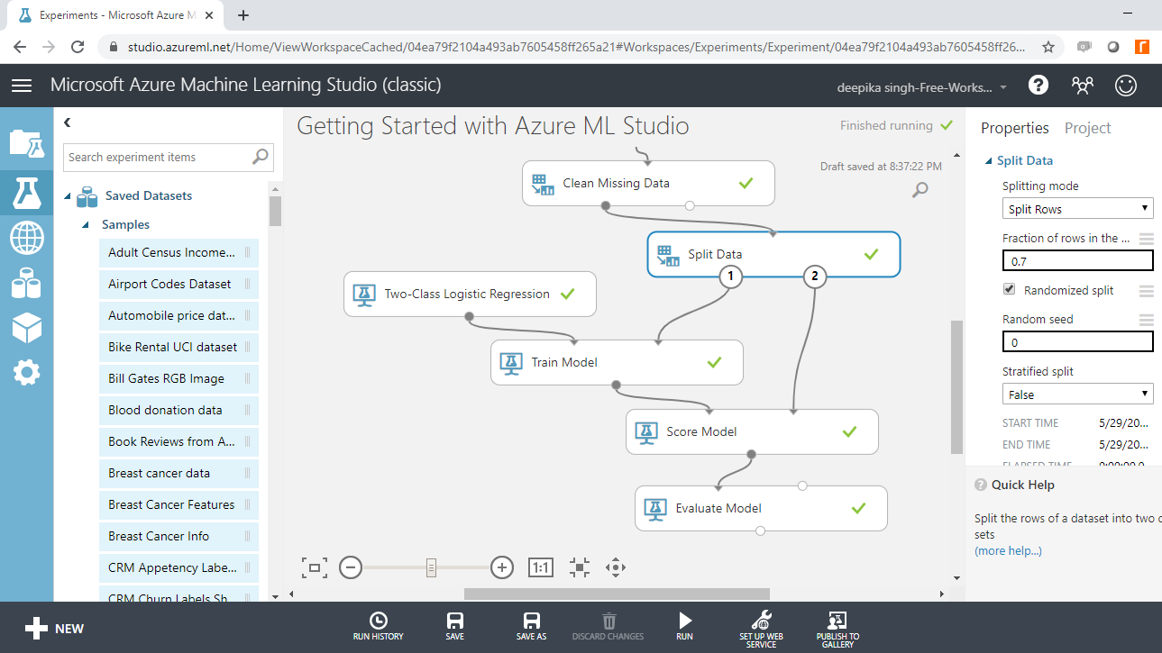
Step Three: Create Train and Test Datasets
You will divide the data into train and test datasets with the Split Data module.
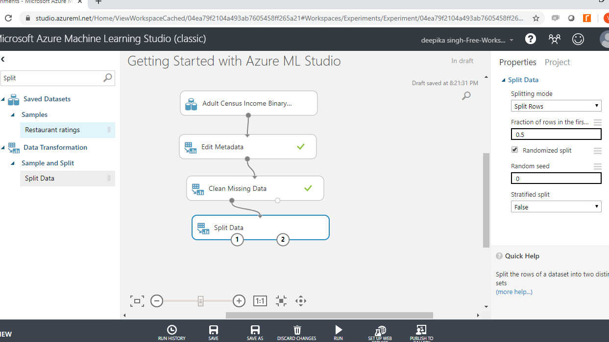
In the Split Data options displayed in the right-hand side of the workspace, change the value under the tab Fraction of rows in the first split to 0.7. This means you are keeping 70% of the data in the training set, while the remaining 30% will remain in the test set. Next, click on the Run tab and select Run selected.
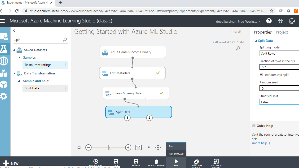
After the execution is complete, the two output ports of the Split Data module will contain the train and test datasets. The left output port contains the train data, while the right output port contains the test dataset.
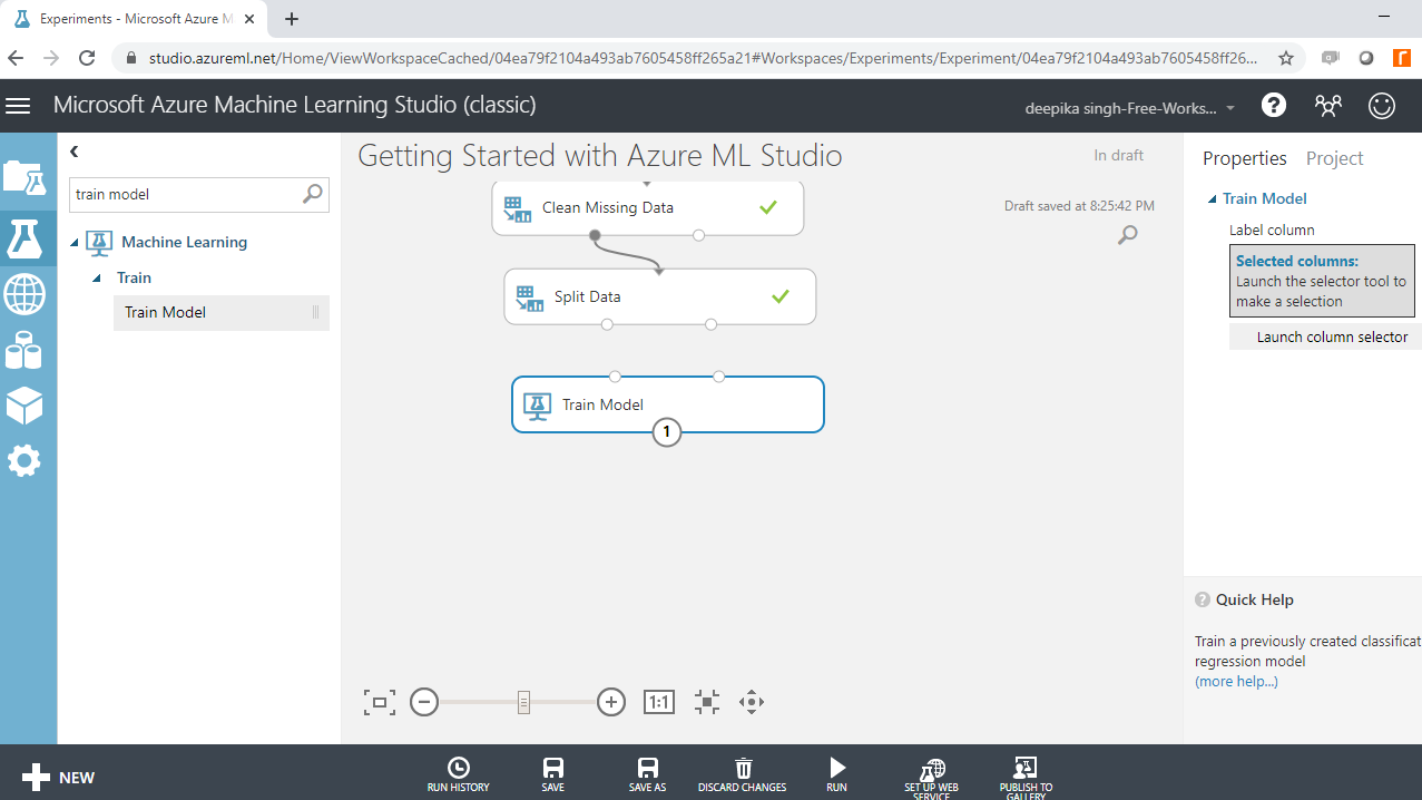
Step Four: Build the Model
The first step is to train the model. Start by dragging the Train Model module into the workspace as shown below.
Since the target variable is binary, you will build a binary classification algorithm. There are many classification algorithms available in ML Studio. You will select and drag the Two-Class Logistic Regression module into the workspace.
Next, connect the right port output from the Split Data module to the left input port of the Train Model module. Also, connect the Two-Class Logistic Regression module with the right input port of the Train Model module.
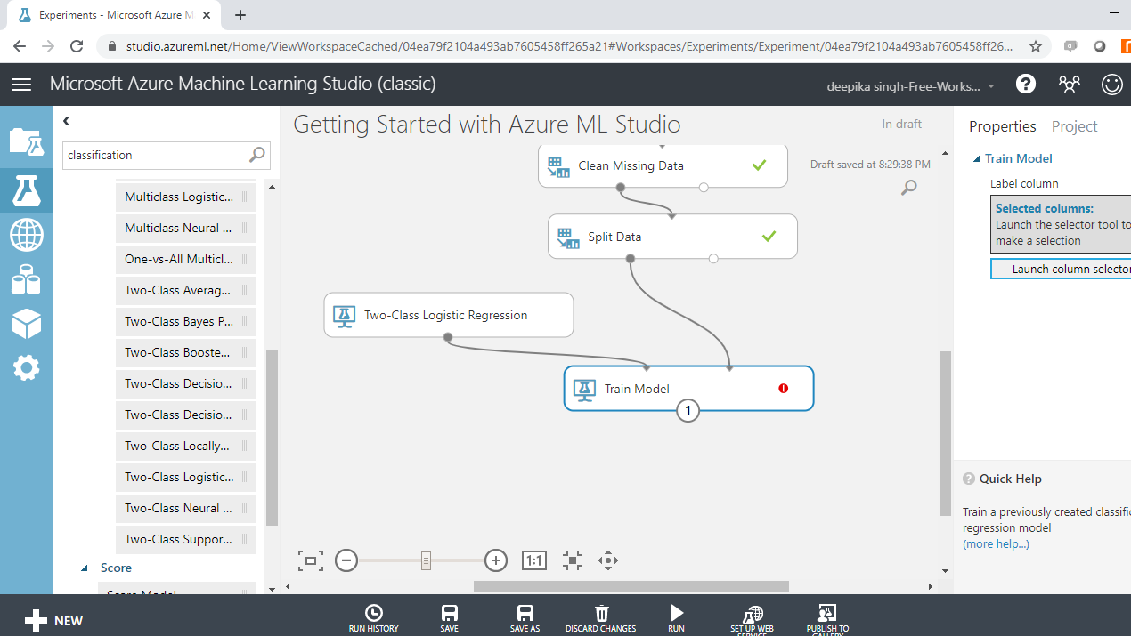
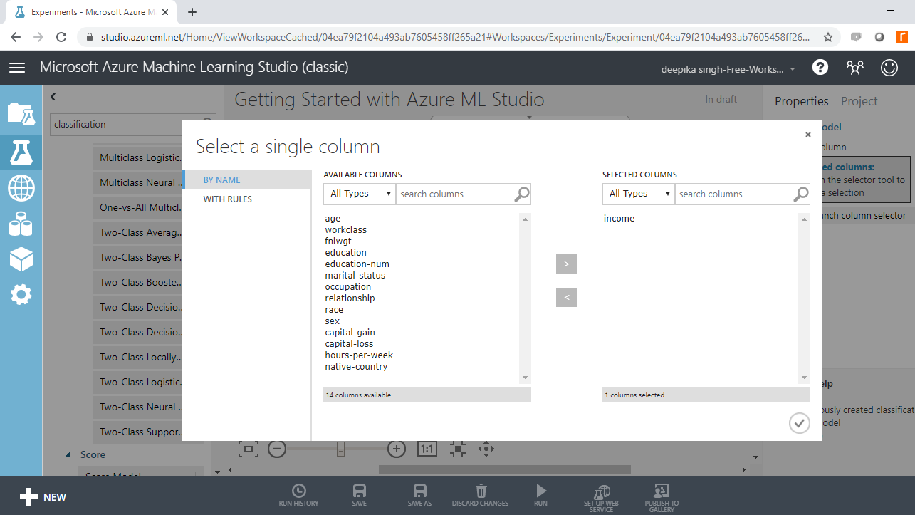
In the output above, you can see that there is a red circle inside the Train Model module that indicates that the setup is not complete. This is because you haven’t specified the target variable yet. To do this, click on Launch column selector, and place the target variable income into the selected columns box, as shown below.
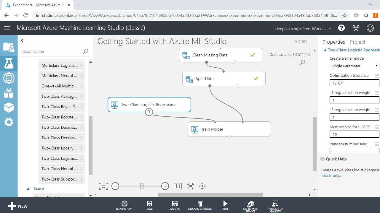
The next step is to specify the parameters of the algorithm. To do this, click on the Two-Class Logistic Regression module and you will see a number of training parameters. Keep the default options or make the changes as per your choice.
The final step in training the model is to click on the RUN tab, and select the Run selected option.
Step Five: Score Test Data
At this point, the model has been built. The next step is to score the test data. Perform the following steps for scoring the test data.:
-
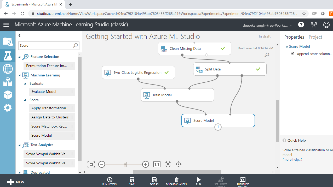
Drag the Score Model module into the workspace.
-
Connect the output port of the Train Model with the left input port of the Score Model module.
-
Connect the right output port of the Split Data module to the right input port of the Score Model module. Note that this connects the test data in the Split Data module with the scoring function.
Your workspace will look as below.
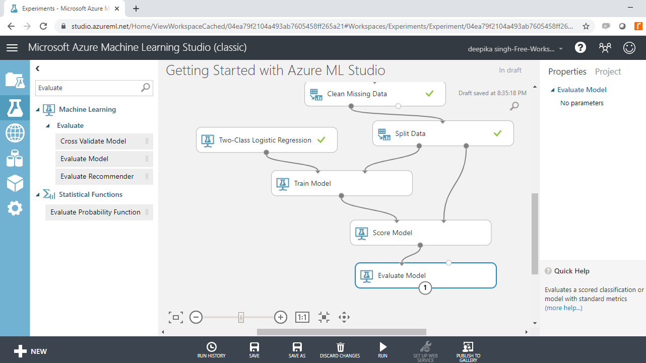
Step Six: Evaluate the Model
You have built the predictive model and generated predictions on the test data. The next step is to evaluate the performance of your predictive model. Drag the Evaluate Model module into the workspace and connect it with the Score Model module as shown below.
Next, click on the Run tab and select Run selected. This will generate the following output.
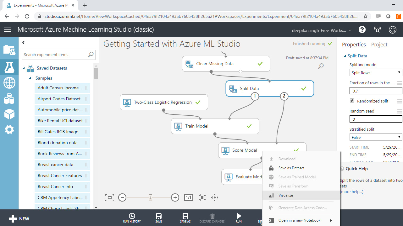
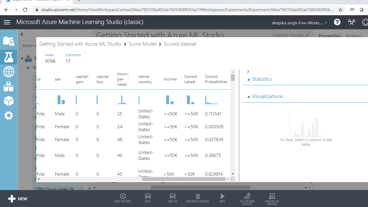
You can start the model evaluation by looking at the scored data. Right click on the output port of the Score Model module and click on the Visualize option.
The above steps will generate the output shown below. You can see that two additional columns have been added to the test data, Scored Labels and Scored Probabilities.
It seems that the model has been able to predict the correct income class well. To quantify this, right click on the output port of the Evaluate Model module and click on the Visualize option.

The result window will open, and you can look at the graph as shown below.
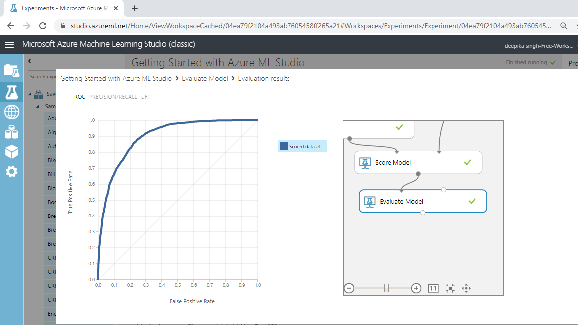
You can scroll down to see the evaluation metrics like precision, recall, accuracy, AUC score and the corresponding threshold.
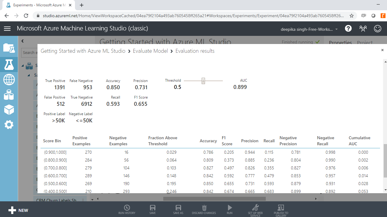
The output above shows that the accuracy of the model is 85% and the AUC score is 0.899, which shows that the model has performed well.
Conclusion
In this guide, you learned about the popular cloud-based machine learning web service, Azure ML Studio. You were introduced to the ML Studio workspace, and learned how to load and prepare the data. You also learned how to build, score, and evaluate the classification algorithm without writing any code. This will get you started in building machine learning models on the cloud using Azure Machine Learning Studio.
Advance your tech skills today
Access courses on AI, cloud, data, security, and more—all led by industry experts.
