Programming Your First Quantum Circuit with IBM Quantum Experience
Nov 17, 2020 • 10 Minute Read
Introduction
As quantum computing gains popularity, various cloud providers are making quantum computers available to the public on their platforms. This guide will focus on the IBM Quantum Experience platform, and show you how to program your first basic quantum circuit.
You'll get to execute that circuit, first using a quantum simulator running on a classical machine, and then on a real quantum device!
First, get acquainted with the platform by going to the homepage. You’ll need to either create a new IBMid or sign in with a third-party provider like GitHub.
Once you’ve logged in, navigate to the Quantum Lab using the left-side navigation bar. This is where your notebooks will live. A notebook refers to a Jupyter Notebook, which is an open source, interactive environment that runs Python code in the browser, and is especially useful for data analysis and equations. These notebook documents use .ipynb for their file extension.
Create a Notebook
Create a new notebook by using the New Notebook + button. You’ll see that some code is already written for you, in what is called a cell. You can run a cell by clicking on it so that it becomes highlighted, then clicking the Run button in the top navigation.
This cell contains default imports that will help you get started. It's important to notice that you are importing Qiskit, which is IBM's open source quantum SDK that uses Python as its programming language. With Qiskit, you can program quantum circuits and run them on simulators or actual quantum systems.
Build the Circuit
Programs written in Qiskit have three main components: build, execute, and analyze. Let's start with the build step.
Initialize
In the following code, you are initializing two qubits and two classical bits, respectively, in a quantum circuit called qc:
      # cell 2
qc = QuantumCircuit(
    2, # quantum register with 2 qubits
    2 # classical register with 2 classical bits
)
Classical bits have two states: 0 and 1. Think of these states as tails and heads on a coin. When programming a classical computer, you are always turning the coin back and forth between these two states.
Similarly qubits, when measured, also exist in the 0 or 1 state. However, before they are measured qubits can also be put into a state of probability called superposition. Imagine this as something like the state the coin is in while it's in midair after a flip. Quantum researchers leverage this unique characteristic of qubits for tasks that require tremendous processing power.
When these qubits and classical bits are initialized, their states are all 0.
While you are measuring the qubits, you are storing the results in the classical bits. The first list in qc.measure() represents the quantum register and the second list represents the classical register. You are mapping one to the other:
      # cell 2
qc.measure([0,1], [0,1])
Execute the Circuit on a Simulator
You have not told your circuit to do anything interesting yet in the build step, but before you get back to that, you need to execute the circuit.
Specify a Simulator
Run your circuit on a quantum simulator first. In this case, that means running optimized C++ code on a classical machine.
Aer is the simulator component of Qiskit, the most frequently used simulator being QasmSimulator because it allows for multi-shot executions:
      # cell 2
simulator = Aer.get_backend('qasm_simulator')
Run the Circuit
Execute the circuit and specify a number of shots (how many times you want to repeat the experiment):
      # cell 2
job = execute(qc, simulator, shots=1000)
Capture Experiment Results
Now, store and format the results of the 1,000 shots that took place:
      # cell 2
result = job.result()
counts = result.get_counts(qc)
print("\nCount:",counts)
All the code so far should be pasted, in order, into the second cell of your notebook. Once it's all there, run the cell. Your output should read:
Count: {'00': 1000}
This means that out of the 1,000 shots you ran, 1,000 times you measured the state 00 (one 0 for each qubit).
Analyze the Circuit
One basic step of circuit analysis is simply drawing it. To do so, add this line to the end of your program in the second cell:
      # cell 2
qc.draw()
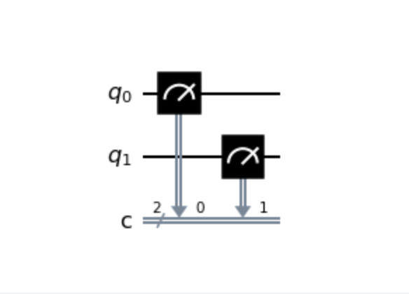
Read a Circuit Diagram
This is a circuit diagram, and you'll see circuit wires for each of the two qubits (annotated with q0 and q1), as well as a double gray line representing the classical bits (annotated with c and a number representing the number of classical bits, in this case two).
Reading from left to right, you'll notice the gauge symbol. This represents the measurement operation. The double gray line coming off the symbol has an arrow pointing to the classical circuit wire and a 0 next to it, meaning you are storing the measurement of qubit q0 in classical bit 0. Moving right, you can see this repeated but for qubit q1 and classical bit 1.
Plot the Results
Create a third cell, and add this line:
      # cell 3
plot_histogram(counts)
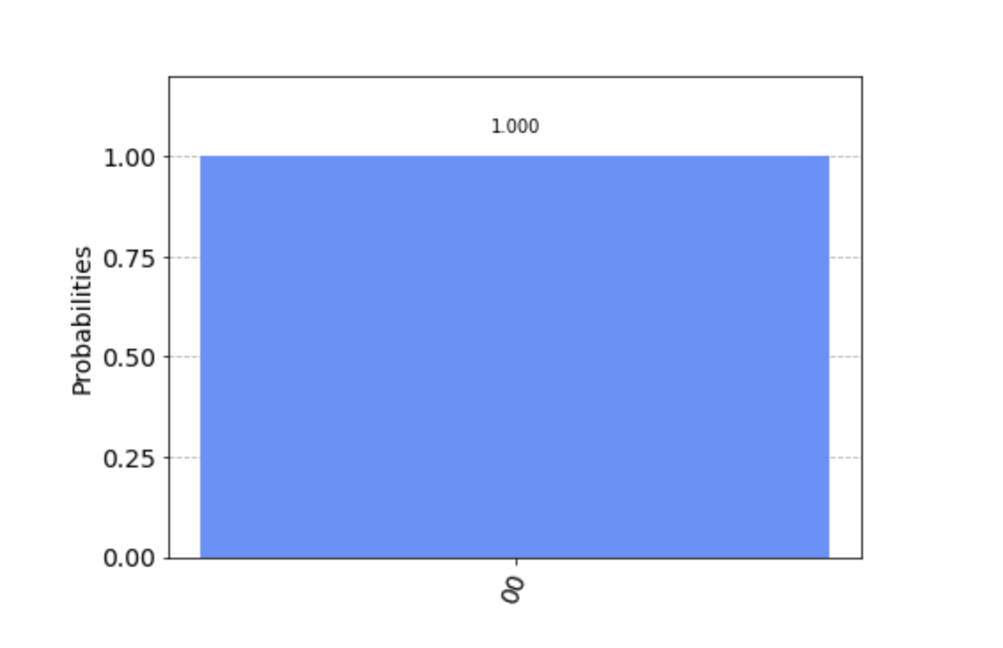
You can see that in this graph, the probability of getting the result 00 is 1.00 or 100%.
Add Quantum Gates
Now you can go back and actually manipulate the qubits using quantum gates.
Classical computers also use classical gates, but in modern programming you generally don't see them because they are abstracted away. A simple classical gate is the NOT gate, which flips a bit from 0 to 1. Some classical gates have related quantum gates, and NOT (also called X or Pauli-X in the quantum world) is one of them.
Before you call qc.measure() in the second cell, add this line:
      # cell 2
qc.h(0)
Here, h stands for Hadamard, which is the name of the gate you are applying, in this case to qubit 0. For now, you can think of the Hadamard gate as putting the coin (a.k.a. qubit) into a state where it is spinning in midair after a flip. The probability of how the coin will land is 50/50. This even split in probability is called uniform superposition.
Run the second cell again. Notice that there are now two results (00 and 01) and they were each measured about 50% of the time. One of the qubits was always measured in the 0 state, while the other was sometimes in the 0 state and sometimes in the 1 state.
You might notice something odd here. You manipulated qubit 0, the first one in the register list. However in the printed results, it's not the first qubit that is variable but the second. This is because when it comes to strings, Qiskit numbers the bits from right to left.
Execution on a Real Quantum System
So far, in this guide, you've only used a simulator to run your circuit. Simulators work great when you are trying estimate how a small number of qubits will behave, and realistically, that is all you will be doing for a while. But what if you wanted to run your experiment on a real quantum device?
For simplicity, start by removing the line with the Hadamard gate. This takes you back to the original experiment, where you saw the result 00 output 100% of the time.
Then, replace the line where you currently define provider in the first cell with the following:
      # cell 1
provider = IBMQ.get_provider(hub='ibm-q')
backends = provider.backends(simulator=False, operational=True)
backend = backends[0]
backend
Run this first cell to see information printed out about the backend you are going to use.
In the second cell, replace the line defining job with the following:
      # cell 2
job = execute(qc, backend, shots=1000)
Now run the second cell (this may take a few minutes).
Do you notice anything interesting? If you view the count output, you'll see that you no longer have just one state that was measured, you have four! Why does this happen?
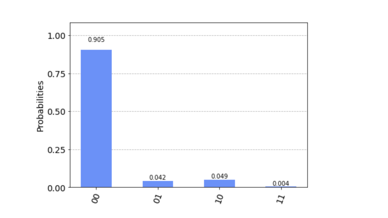
Quantum systems are extremely sensitive and are prone to interference from their environment, which has an impact on the state of the qubits. This is also why you should run the experiment many times—if you ran it just one time, your result could be very inaccurate.
If you want to see information about the job you just ran, go to the Results tab in the left-side navigation.
Conclusion
Now that you've seen how a basic circuit works, you can start building on it with more qubits and more quantum gates. To learn more about quantum computing in general, check out my Pluralsight guide covering the basic principles, as well as the IBM docs.
Advance your tech skills today
Access courses on AI, cloud, data, security, and more—all led by industry experts.
