Visualizing Text Data using Word Cloud in Azure Machine Learning Studio

Word clouds are an excellent way to analyze text data through visualization in the form of tags, or words, based on their frequency.

Oct 12, 2020 • 10 Minute Read

Subscribe to the newsletter

Introduction

The amount of text data has grown exponentially in recent years, resulting in an ever-increasing need to analyze the massive amounts of such data. Word clouds provide an excellent option to analyze text data through visualization in the form of tags, or words, where the importance of a word is explained by its frequency. In this guide, you will learn how to visualize text data using the word cloud feature in Azure Machine Learning Studio.

Data

In this guide, you will work with Twitter data of the Bollywood movie Rangoon. The movie was released on February 24, 2017, and the tweets were extracted on February 25. These tweets have been stored in a file named movietweets. The data contains tweets in rows, and the column you will consider is the text variable, which contains the tweet. Start by loading the data into the workspace.

Loading Data

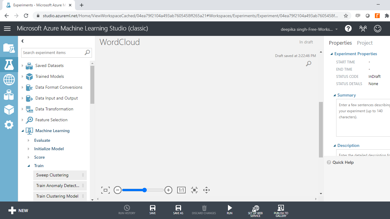
Once you have logged into your Azure Machine Learning Studio account, click the EXPERIMENTS option, listed on the left sidebar, followed by the NEW button.

Next, click on the blank experiment and a new workspace will open. Give the name WordCloud to the workspace.

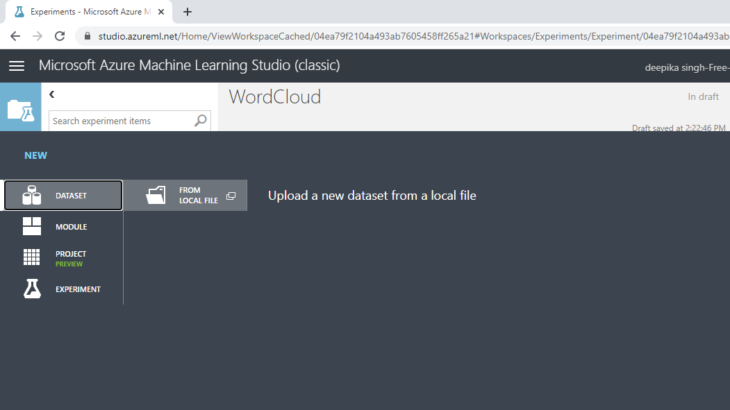
Next, load the data into the workspace. Click NEW, and select the DATASET option shown below.

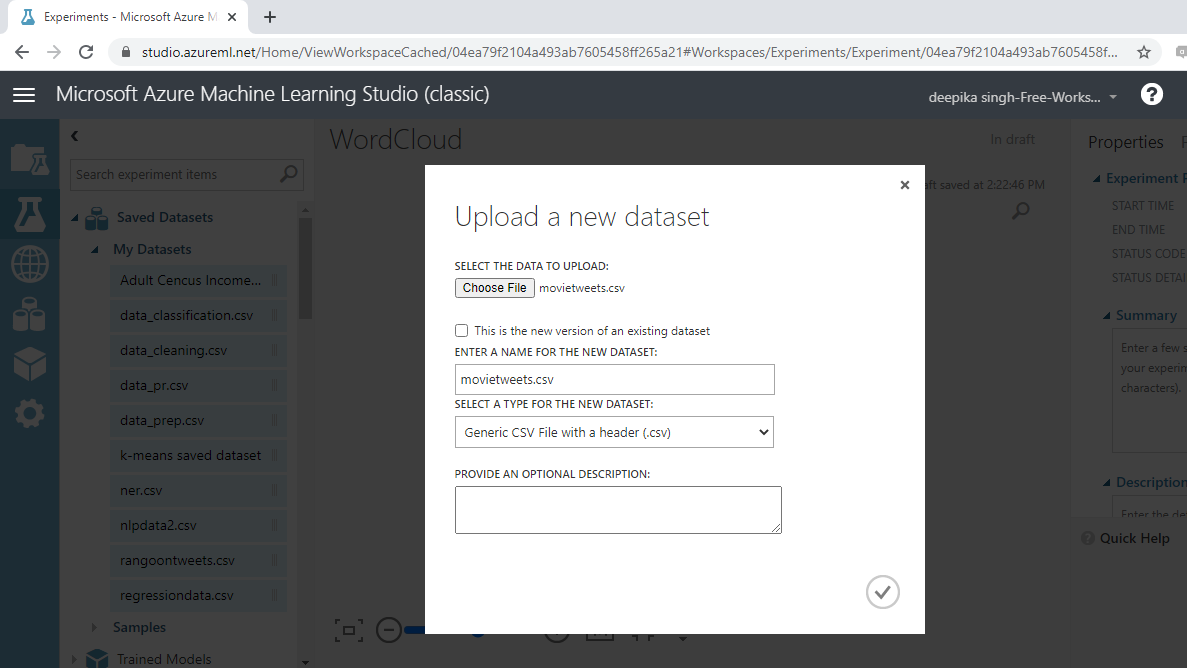
The selection above will open a window, shown below, which can be used to upload the dataset from the local system.

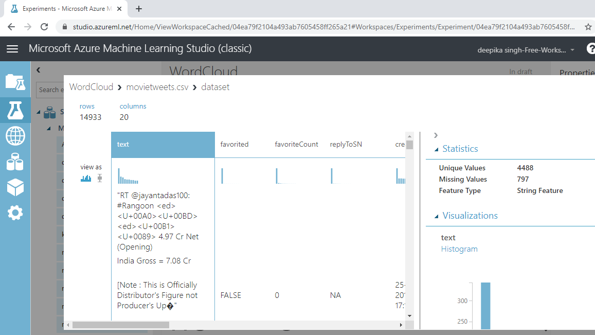
Once the data is loaded, you can see it in the Saved Datasets option. The file name is movietweets.csv. The next step is to drag it from the Saved Datasets list into the workspace. To explore this data, right-click and select the Visualize option, as shown below.

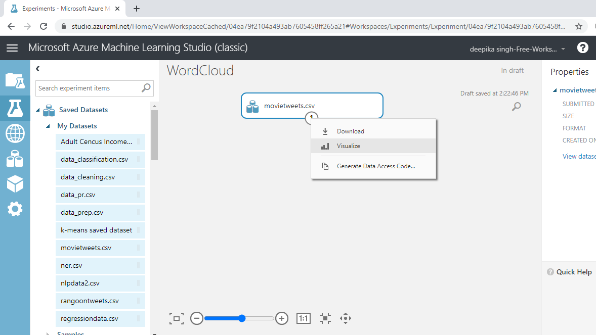
You can see there are 14933 rows and 20 columns.

Text Preprocessing

It is important to pre-process text before you visualize it with a word cloud. Common pre-processing steps include:

Remove punctuation: The rule of thumb is to remove everything that is not in the form x,y,z.
Remove stop words: These are unhelpful words like "the", "is", or "at". These are not helpful because the frequency of such stop words is high in the corpus, but they don't help in differentiating the target classes. The removal of stop words also reduces the data size.
Conversion to lowercase: Words like "Clinical" and "clinical" need to be considered as one word. Hence, these are converted to lowercase.
Stemming: The goal of stemming is to reduce the number of inflectional forms of words appearing in the text. This causes words such as “argue,” "argued," "arguing," and "argues" to be reduced to their common stem, “argu”. This helps in decreasing the size of the vocabulary space.

The Preprocess Text module is used to perform these and other text cleaning steps. Search and drag the module into the workspace. Connect it to the data as shown below.

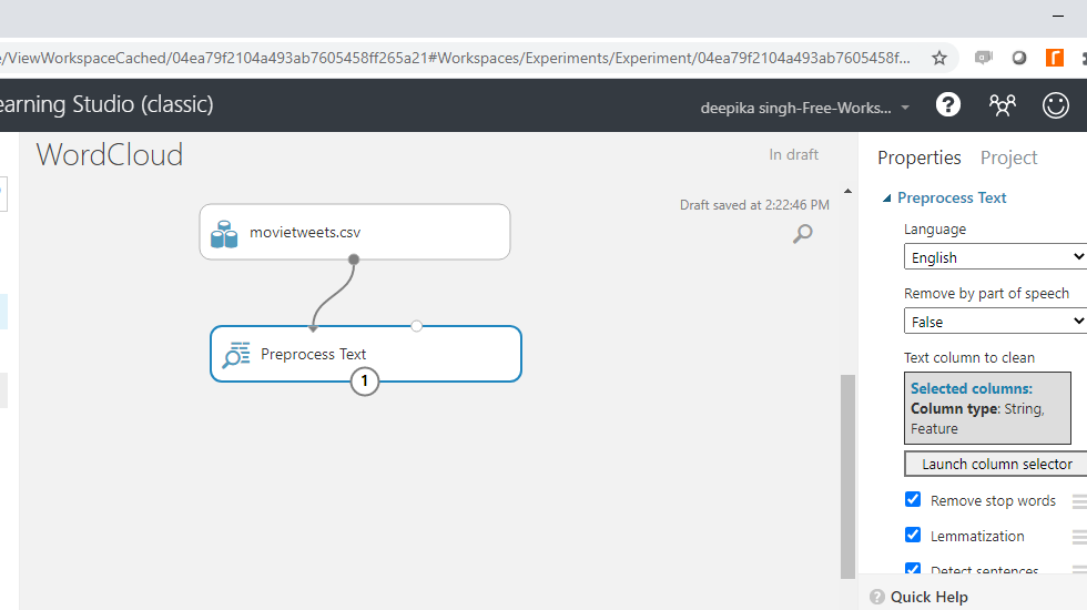
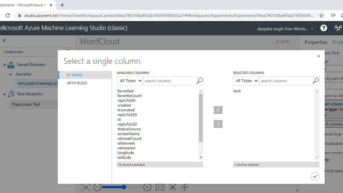
You must specify the text variable to be pre-processed. Click on the Launch column selector option, and select the text variable.

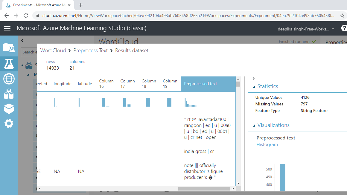
Run the experiment and click Visualize to see the result. The Preprocessed text variable contains the processed text.

Build a Word Cloud

You have performed the pre-processing step, and the corpus is ready to be used for building a word cloud. You will use the R programming language to generate the word cloud. The Execute R Script module is used to execute R codes in the machine learning experiment.

To begin, search and add the Execute R Script module to the experiment. Next, connect the data to the first input port (left-most) of the module.

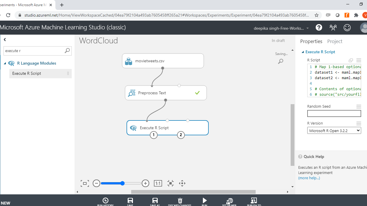
Click on the module and under the Properties pane. You will see the option of writing your R script. Enter the code as shown below.

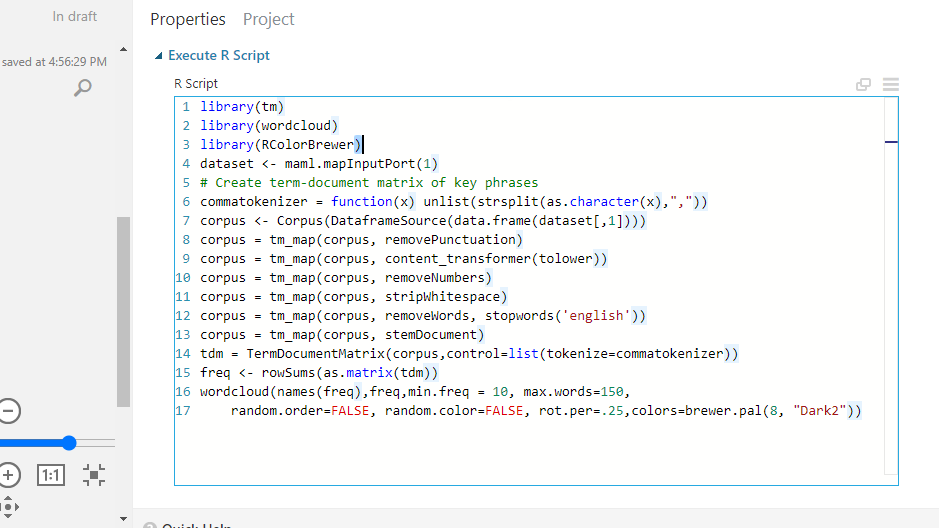
You can also copy the code below.

      #lines 1 to 4

library(tm)
library(wordcloud)
library(RColorBrewer)
dataset <- maml.mapInputPort(1)

# lines 5 to 12 – text preprocessing 

commatokenizer = function(x) unlist(strsplit(as.character(x),","))
corpus <- Corpus(DataframeSource(data.frame(dataset[,1])))
corpus = tm_map(corpus, removePunctuation)
corpus = tm_map(corpus, content_transformer(tolower))
corpus = tm_map(corpus, removeNumbers)
corpus = tm_map(corpus, stripWhitespace)
corpus = tm_map(corpus, removeWords, stopwords('english'))
corpus = tm_map(corpus, stemDocument)

# lines 13 and 14 - Create term-document matrix, frequency 

tdm = TermDocumentMatrix(corpus,control=list(tokenize=commatokenizer))
freq <- rowSums(as.matrix(tdm))

# line 15

wordcloud(names(freq),freq,min.freq = 10, max.words=150, 
random.order=FALSE, random.color=FALSE, rot.per=.25,colors=brewer.pal(8, "Dark2"))
    

Code Explanation

In the code above, the first three lines of code load the required libraries. The fourth line creates a dataframe, dataset1, which is mapped to the first input port with the function,mam1.mapInputPort().

Line of codes from five to twelve perform further refining on the earlier preprocessed text data with the tm_map function. The next two lines create the document term matrix and store the frequency of words in the freq object. Finally, the wordcloud() function is used to build the word cloud. The major arguments of this function are given below.

min.freq: An argument which ensures that words with a frequency below min.freq will not be plotted in the word cloud.
max.words: The maximum number of words to be plotted.
random.order: An argument that specifies plotting of words in random order. If false, the words are plotted in decreasing frequency.
rot.per: The proportion of words with 90-degree rotation (vertical text).
colors: An argument that specifies the color of words from least to most frequent.

The above arguments have been provided in the wordcloud() function. Once you have set up the experiment, the next step is to run it.

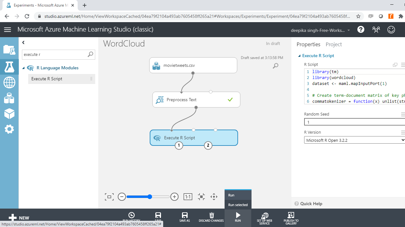
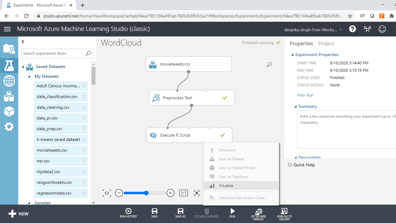
On successful completion, you can see the green tick in the module.

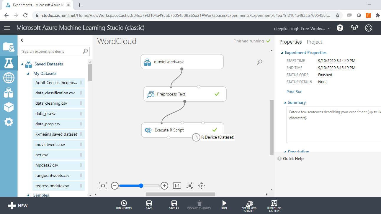
Right-click and select Visualize to look at the output.

The following output is displayed. The word cloud generated shows that the words are plotted in decreasing frequency, which means that the most frequent words are in the center of the word cloud, and the words with lower frequency are farther away from the center.

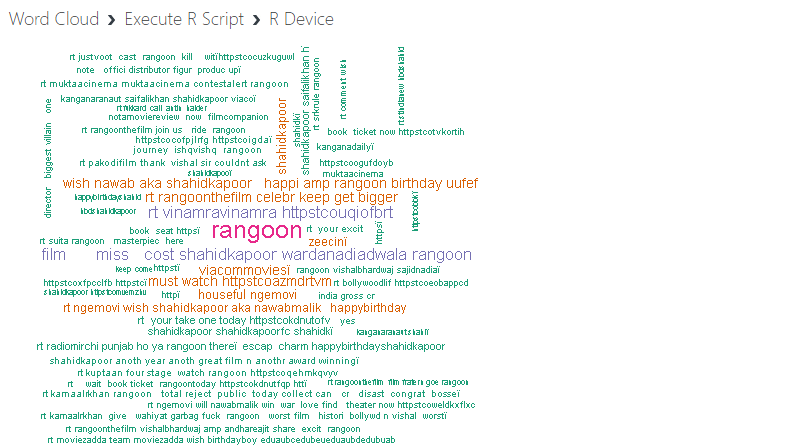
You can see that the word "rangoon" is at the center of the word cloud, which makes sense as it was the name of the movie. Another interesting word is "miss," because the name of the central character in the movie was Miss Julia. This way, you can analyze the important words in a text corpus using a word cloud.

Conclusion

Word clouds are very useful in sentiment analysis as they highlight the key words in text. This has application in Twitter, Facebook, and other social media analytics tasks. Word clouds are also applied to build marketing campaigns or plan promotional advertisements where significant words are used.

In this guide, you learned how to visualize text data using Word Cloud in Azure ML Studio. You can learn more on text visualization with guides on other technologies like Python and R.

To learn more about data science and machine learning using Azure Machine Learning Studio, please refer to the following guides: